
Script
📚 Catalogue
De-meta-analysis
It is also possible to exclude the effects of one cohort from GWAS summary statistics, using a de-meta-analysis:
\[\hat {\beta}_{DE-META} = \hat{\beta}_{META} - SE^2_{\hat{\beta}_{DE-META}} \sum_c \frac{\hat {\beta}_{c} - \hat{\beta}_{META} }{SE^2_{\hat{\beta}_{c}}}\] \[SE_{\hat{\beta}_{DE-META}} = \sqrt{\frac{1}{\frac{1}{SE^2_{\hat{\beta}_{META}}}-\sum_c \frac{1}{SE^2_{\hat{\beta}_{c}}}}}\]🧠 Let’s we implement using R script
rescale_b_se <- function(gwas, case, control){
  names(gwas) = c("SNP","A1","A2","freq","b","se","P","N")
  n_eff       = as.integer(4*case*control/(case + control))
  p           = gwas$freq
  z           = gwas$b / gwas$se
  se          = 1/sqrt(2*p*(1-p)*(n_eff+z^2))
  b           = z*se
  gwas$b      = b
  gwas$se     = se
  gwas$N      = n_eff

  return(gwas)
}

de_meta <- function(meta, sub_c){
  if (!requireNamespace("logger", quietly=TRUE)){ install.packages("logger") }
  lapply(c("dplyr","data.table","logger"), function(pkg) suppressWarnings(library(pkg,character.only=TRUE)))

  log_info("Start to check the input meta...")
  log_info("Start to check SNP effect size")
  if(any(meta$beta_meta == 0)){
    Delmeta = meta[meta$beta_meta == 0, ]
    log_info(paste("The meta file contained", nrow(Delmeta), "SNPs that effect size = 0"))
    meta = meta[!(SNP %in% Delmeta$SNP)]
    log_info("We will delete these SNPs")
  }else{ log_info("No SNPs effect size = 0") }

  log_info("Start to check P value")
  if(any(meta$p > 1 | meta$p < 0)){
    Delmeta = meta[meta$p > 1 | meta$p < 0, ]
    log_info(paste("The meta file contained", nrow(Delmeta), "SNPs that Pvalue > 1 or < 0"))
    meta = meta[!(SNP %in% Delmeta$SNP)]
    log_info("We will delete these SNPs")
  }else{ log_info("No SNPs Pvalue > 1 or < 0") }

  log_info("Start to check the input sub_c...")
  log_info("Start to check SNP effect size")
  if(any(sub_c$beta_c == 0)){
    Delmeta = sub_c[sub_c$beta_c == 0, ]
    log_info(paste("The sub_c file contained", nrow(Delmeta), "SNPs that effect size = 0"))
    sub_c = sub_c[!(SNP %in% Delmeta$SNP)]
    log_info("We will delete these SNPs")
  }else{ log_info("No SNPs effect size = 0") }

  log_info("Start to merge the meta and sub_c by SNP")
  combined_data <- merge(meta,sub_c,by="SNP")

  log_info("Start to keep meta only SNPs")
  meta_only <- meta[meta$SNP %in% setdiff(meta$SNP,sub_c$SNP), ]
  meta_only [, n_meta := n_meta - unique(sub_c$N)]
  setDT(meta_only)
  setnames(meta_only, c("SNP","A1","A2","freq","b","se","p","N"))
  log_info(paste("There were", nrow(meta_only), "SNPs only occured in meta"))

  log_info("Start to fix the effect allele in meta and sub_c")
  combined_data[, beta_c := ifelse((A1_m==A1_c & A2_m==A2_c),beta,ifelse(A1_m==A2_c & A2_m==A1_c,-beta,NA_real_))]
  if(any(is.na(combined_data$beta_c))) {
    Deldt = subset(combined_data, is.na(combined_data$beta_c))
    log_info(paste("There were", nrow(Deldt), "SNPs have unmatched alleles, will delete these SNPs!"))
    log_info(paste("In these SNPs, the lowest P value is", min(Deldt$p)))
    combined_data = combined_data[!(SNP %in% Deldt$SNP)]
  }

  log_info("Start to demeta SNP effect size and se")
  se_meta_mean <- mean(combined_data$se_meta, na.rm=TRUE)
  combined_data[, se_demeta := fifelse((1/se_meta^2 - 1/se_c^2) > 0, sqrt(1/(1/se_meta^2 - 1/se_c^2)),se_meta_mean)]
  combined_data[, beta_demeta := beta_meta-se_demeta^2 * (beta_c-beta_meta)/se_c^2]


  if (any(combined_data$beta_demeta == 0)) {
    log_info("There may be generate zero beta after demeta!")
    Deldt = combined_data[combined_data$beta_demeta == 0, ]
    log_info(paste("There were", nrow(Deldt), "SNPs has been deleted casued by the demeta value is zero!"))
    combined_data = combined_data[!(SNP %in% Deldt$SNP), ]
  }

  log_info("Start to create effect N of demeta")
  combined_data[, N_eff := n_meta - N]

  common_SNP <- combined_data[, c("SNP","A1_m","A2_m","freq","beta_demeta","se_demeta","p","N_eff")]
  setDT(common_SNP)
  setnames(common_SNP, c("SNP","A1","A2","freq","b","se","p","N"))

  log_info("Start to combine meta only SNPs and demeta SNPs to one")
  outfile <- rbind(common_SNP,meta_only)

  log_info("Start to calculate P value based on beta and se")
  outfile$p <- 2 * (1 - pnorm(abs(outfile$b / outfile$se)))

  log_info("Demeta analysis is completed!")
  return(outfile)
}
🧪 Just use it as follow: in this case, we using hapmap 3 SNP to do de-meta
library(data.table)
hm3 = fread("listHM3.txt", col.names="SNP")

meta = fread("ARHL_MVP_AJHG_BBJ_reformatMETAL.txt")
meta_hm3 = merge(meta, hm3, by="SNP")
names(meta_hm3) = c("SNP","A1_m","A2_m","freq","beta_meta","se_meta","p","n_meta")

## rescale beta se for sub cohort data
sub_c = fread("2247_1.v1.1.fastGWA", select=c("SNP","A1","A2","AF1","BETA","SE","P","N"))
sub_c_hm3 = merge(sub_c, hm3, by="SNP")

re_sub_c_hm3 = rescale_b_se(sub_c_hm3, 114318, 323449)
names(re_sub_c_hm3) = c("SNP","A1_c","A2_c","freq_c","beta","se_c","p_c","N")

# run demeta for meta and ajhg
demeta_meta_hm3 = de_meta(meta_hm3, re_sub_c_hm3)


out_meta_demeta_hm3 = demeta_meta_hm3[which(demeta_meta_hm3$N > 100000),]
fwrite(out_meta_demeta_hm3, file="Demeta_raw_hm3.txt", sep="\t")
SMR plot for multi tissue in one fig
🧠 When you want draw multi tissue SMR result in one fig, this script will meet your require
#***********************************************#
# File   :   CreateMultiTissueSMRPlotData.r     #
# Time   :   14Apr2025 18:00:51                 #
# Author :   Loren Shi                          #
# Mails  :   crazzy_rabbit@163.com              #
# link   :   https://github.com/Crazzy-Rabbit   #
#***********************************************#
ExtractProbe <- function(QTL, chr, centerbp, window=10e5, probes, tissue){
	# 1.generate probe list in range
	start = centerbp - window;
	end = centerbp + window;
	QTLepi = read.delim(paste0(QTL,".epi"),head=F)
	QTLindex = which(QTLepi$V1==chr & QTLepi$V4>=start & QTLepi$V4<=end)
	QTLout = paste0(dir, "/", basename(QTL), "_", probes) # probe list filename
	write.table(QTLepi[QTLindex,2], QTLout,col.names=FALSE,row.names=FALSE,sep="\t",quote=FALSE)

	# 2.extract besd files
	SMR="~/software/smr-1.3.1/smr"
    system(paste(SMR, "--beqtl-summary", QTL,
                    "--chr", chr,
                    "--extract-probe", QTLout,
                    "--thread-num 10",
					"--make-besd",
					"--out", QTLout))

	# 3.update the probe names in epi file, probe as tissue: ENSG00000122786
	epi = read.table(paste0(QTLout, ".epi"), head=FALSE)
	epi$V2 = paste0(tissue, "-", epi$V2)
	write.table(epi, paste0(QTLout, ".epi"), col.names=FALSE,row.names=FALSE,sep="\t",quote=FALSE)

	return(QTLout)
}

CreateMultiTissueSMRPlotDt <- function(esi_profix_list, tissue, probes, ref, gwas, windows=2000, outprefix){
    library(data.table)
	# the loop to match esi file pos
	esi_list = lapply(esi_profix_list, function(prefix) {
		fread(paste0(prefix, ".esi"))
	})
	n=length(esi_list)
	esiSet = unique(do.call(rbind, esi_list))
	snpSet = unique(unlist(lapply(esi_list, function(x) x$V2)))
	idx = match(snpSet, esiSet$V2)
	refSet = data.frame(snpSet, A1=esiSet$V5[idx], A2=esiSet$V6[idx])
    idx_list = lapply(esi_list, function(x) match(x$V2, esiSet$V2))

	for (i in seq_along(esi_list)) {
		idxs = idx_list[[i]]
		esi_list[[i]]$V5 = refSet$A1[idxs]
		esi_list[[i]]$V6 = refSet$A2[idxs]
		outfile = paste0(esi_profix_list[i], ".esi")
		write.table(esi_list[[i]],outfile,col.names=FALSE,row.names=FALSE,sep="\t",quote=FALSE)
	}

	# merge multi tissue besd file
	SMR="~/software/smr-1.3.1/smr"
	genelist="~/script/plot_smr/glist_hg19_refseq.txt"

    flist = paste0(outprefix, ".list")
	writeLines(esi_profix_list, flist)
    system(paste(SMR, "--besd-flist", flist,
                "--make-besd",
				"--out", outprefix))

    # extract plot dt
	new_probe = paste0(tissue, "-", probes)
    system(paste(SMR, "--beqtl-summary", outprefix,
				"--gwas-summary", gwas,
				"--bfile", ref,
				"--plot",
				"--diff-freq-prop 0.2",
				"--probe", new_probe,
				"--probe-wind", windows,
				"--gene-list", genelist,
				"--out", outprefix))

}
please replace the SMR dir when you use this script ! ! !
🧪 Example for using:
# index for below used
reference="~/Wulab_share/1000GenomePhase3_Ref_hg37/g1000_eas/g1000_eas"
Adipose_Subcutaneous="/~/Wulab_share/SMR_xQTL_besd/eqtl_all_tissue_GTEx/Adipose_Subcutaneous"
Skin_Sun_Exposed_Lower_leg="~/Wulab_share/SMR_xQTL_besd/eqtl_all_tissue_GTEx/Skin_Sun_Exposed_Lower_leg"
gwas='~/Wulab_project/NSOC/NSOC_filter_maf.txt'
dir="~/Wulab_project/NSOC/CALD1_eQTL"

source("~/script/plot_smr/CreateMultiTissueSMRPlotData.r")
# extract target probe and update the probe name in new epi file
file_idx1 = ExtractProbe(QTL=Adipose_Subcutaneous, chr=7, centerbp=134.429e6, window=10e5,
                        probes="ENSG00000122786", tissue="Adipose_Subcutaneous")
file_idx2 = ExtractProbe(QTL=Skin_Sun_Exposed_Lower_leg, chr=7, centerbp=134.429e6, window=10e5,
                        probes="ENSG00000122786", tissue="Skin_Sun_Exposed_Lower_leg")

# match pos in each esi file and merge these besd file, then generate multi tissue SMR plot file
esi_profix_list=c(file_idx1, file_idx2)
CreateMultiTissueSMRPlotDt(esi_profix_list=esi_profix_list, tissue="Adipose_Subcutaneous", probes="ENSG00000122786",
                        ref=reference, gwas=gwas, windows=2000, outprefix="multiTissue_eQTL_CALD1")


#====================================#
#  plot
#====================================#
source("E:/Shi/ALL_of_my_Job/WCH_script/SMRplot/plot_epiSMR_LorenShi.r")

SMRData = ReadSMRData("multiTissue_eQTL_CALD1.Adipose_Subcutaneous-ENSG00000122786.txt")

pdf('CALD1_multi_tissue.ENSG00000122786.pdf',width = 10,height = 15)
SMRLocusPlot(data=SMRData, smr_thresh=2.44e-4, heidi_thresh=0.01, plotWindow=400, max_anno_probe=4,
            probeNEARBY=c("Skin_Sun_Exposed_Lower_leg-ENSG00000122786"), highlight=c("rs17168118","rs10488465", "rs4732060"),
            anno_self=T, annoSig_only=F, epi_plot=TRUE, funcAnnoFile = "E:/Shi/plot_smr/funcAnno.RData")
dev.off()
Manhattan plot for GWAS or others
🧠 When you want draw Manhattan plot, follow scripts will meet your require
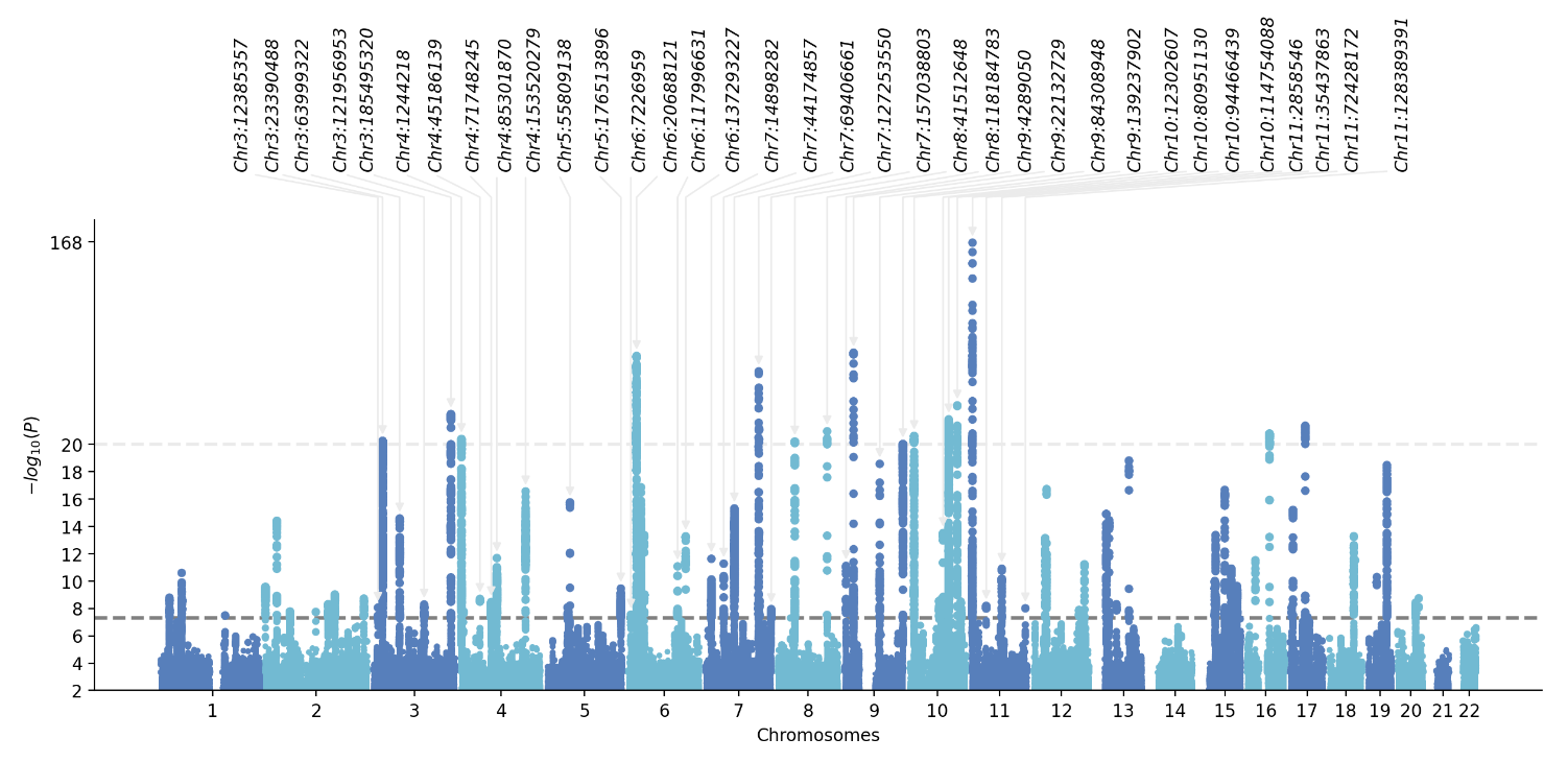
1 gwaslab
More detail please see gwaslab
import gwaslab as gl
import pandas as pd
import matplotlib.pyplot as plt

# 1. data read
gwas = gl.Sumstats("ARHL_MVP_AJHG_BBJ_reformatMETAL_addchr.gz",
                   snpid="SNP",
                   chrom="CHR",
                   pos="POS",
                   ea="A1",
                   nea="A2",
                   eaf="freq",
                   beta="beta",
                   se="SE",
                   p="p",
                   n="N",
                   build="19")

# 2. plot manhattan with annota
df = pd.read_csv("novel_snp_ARHL.txt", sep="\t")
anno_list = df["SNP"].tolist()

gwas.plot_mqq(mode="m", skip=0, sig_line_color="red", fontsize=12, marker_size=(5,5),
              anno="GENENAME", anno_style="expand", anno_set=anno_list, anno_fontsize=12, repel_force=0.01, arm_scale=1,
              xtight=True, ylim=(0,38), chrpad=0.01, xpad=0.05, # cut=40, cut_line_color="white",
              fig_args={"figsize": (18, 5), "dpi": 500},
              save="mqq_plot.png", save_args={"dpi": 500}, check=False, verbose=False)
2 CMplot
More detail please see CMplot
#  file columns should has SNP CHR BP P
args        <- commandArgs(TRUE)
ptype       <- args[1]
infile      <- args[2]
outname     <- args[3]

library(CMplot)
library(data.table)
library(dplyr)

data        <- fread(infile) %>% filter(complete.cases(.))
if (!all(c("SNP", "CHR", "BP", "P") %in% names(data))) stop("The file you provide not contains columns SNP, CHR, BP, and P")
pltdt       <- subset(data, select=c(SNP, CHR, BP, P))
plt_filter  <- na.omit(pltdt[pltdt$P > 0 & pltdt$P < 1, ])  # remove na and keep 0 < p < 1
my_color    <- c('#1B2C62', '#4695BC')

manhattan   <- function (plt, out, ylim=NULL, dpi=500, height=5, width=15, highlight=NULL, highlight.pch=19) {
  CMplot(plt, type="p", plot.type="m", LOG10=TRUE, ylim=ylim,
       file="jpg", file.name=out, file.output=TRUE, dpi=dpi,
       threshold=5e-8, threshold.col="red", threshold.lwd=2, threshold.lty=2,
       highlight=highlight, highlight.pch=highlight.pch,
       col=my_color, band=0,
       cex=0.6, signal.cex=0.6, height=height, width=width)
}

qqplot    <- function(plt, out, dpi=500, width=10, height=10){
CMplot(plt, plot.type="q", LOG10=TRUE, file="jpg", file.name=outname, dpi=dpi,
       file.name=out, verbose=TRUE, cex=0.8, signal.cex=0.8, width=width, height=height,
       threshold.col="red", threshold.lty=2, conf.int=TRUE, conf.int.col=NULL, file.output=TRUE)
}

if (ptype == "manhattan") {
       if (any(-log10(plt_filter$P) > 50)){
              manhattan(plt=plt_filter, out=outname, ylim=c(0, 50))
       } else {
            manhattan(plt=plt_filter, out=outname)
       }
} elseif (ptype == "qqplot") {
       qqplot(plt=plt_filter, out=outname)
}
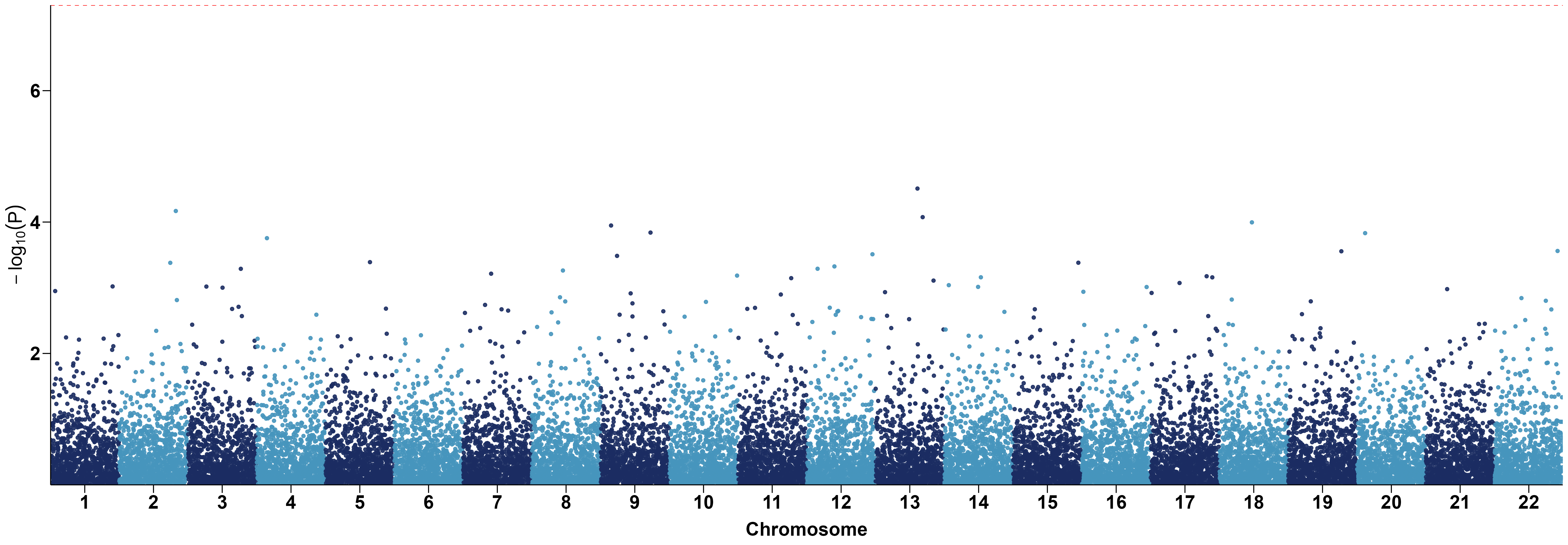
3 ggplot2
library(data.table)
library(ggplot2)
library(dplyr)

dt = fread(infile)[, c("CHR", "BP", "P")]
chr_lengths <- dt %>%
  group_by(CHR) %>%
  summarise(chr_len = max(BP))

data <- dt %>%
  arrange(CHR, BP) %>%
  mutate(chr_cumsum = cumsum(c(0, head(chr_lengths$chr_len, -1)))[CHR]) %>%
  mutate(BPcum = BP + chr_cumsum)

axis_set <- data %>%
  group_by(CHR) %>%
  summarise(center = (max(BPcum) + min(BPcum)) / 2)

p = ggplot(data, aes(x=BPcum, y=-log10(P), color=factor(CHR))) +
  geom_point(alpha=0.9) +
  geom_hline(yintercept=-log10(5e-8), color="red", linetype="dashed") +
  scale_color_manual(values=rep(c("#1B2C62", "#4695BC"), 22)) +
  scale_x_continuous(label=axis_set$CHR,
  	                 breaks=axis_set$center,
                     expand=c(0, 0)) +
  scale_y_continuous(expand=c(0, 0)) +
  labs(x="Chromosome", y=expression(-log[10](P))) +
  theme_classic() +
  theme(legend.position="none",
  	    axis.text.x = element_text(face="bold", size=20, color="black"),
        axis.text.y = element_text(face="bold", size=20, color="black"),
        axis.title.x = element_text(face="bold", size=20, margin=margin(t=10), color="black"),
        axis.title.y = element_text(face="bold", size=20, margin=margin(t=10), color="black"),
        axis.line = element_line(color="black"),
        axis.ticks = element_line(color="black"),
        axis.ticks.length = unit(0.3, "cm"))
ggsave("my.png", p, height = 8, width = 23, dpi=300)
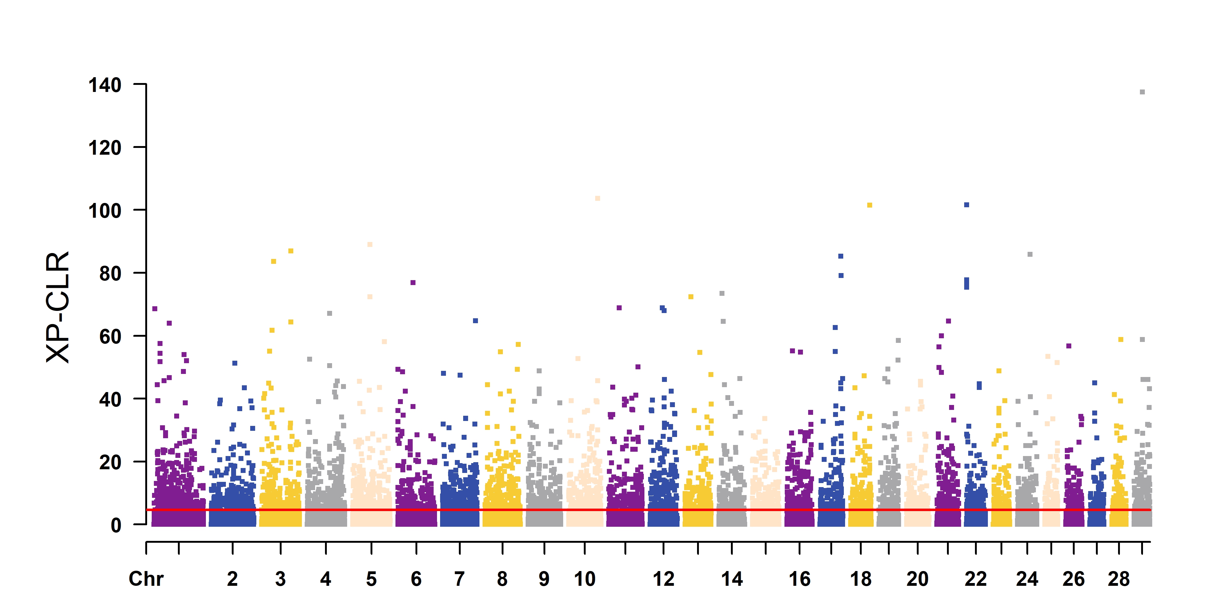
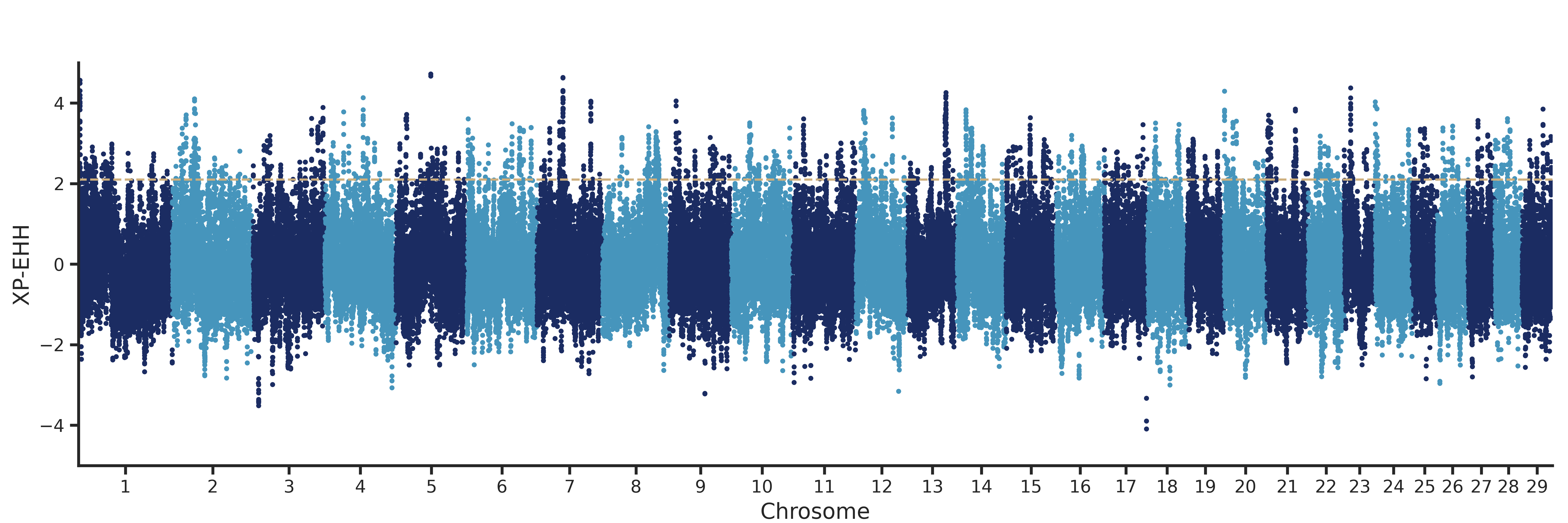
4 Python
# -*- coding: utf-8 -*-
"""
Created on Mon Jan 15 20:28:05 2018

@author: Caiyd
"""

import json
import click
CONTEXT_SETTINGS = dict(help_option_names=['-h', '--help'])
import numpy as np
import pandas as pd
import matplotlib
matplotlib.use('Agg')
import matplotlib.pyplot as plt
import seaborn as sns
from itertools import cycle


def load_allchrom_data(infile, chr_col, loc_col, val_col, log_trans, neg_logtrans):
    """
    infile contain several chromosomes
    """
    df = pd.read_csv(infile,
                     sep='\t',
                     usecols = [chr_col, loc_col, val_col],
                     dtype={chr_col: str,
                            loc_col: float,
                            val_col: float})
    if log_trans:
        df.loc[:, val_col] = np.log10(df[val_col].values)
    elif neg_logtrans:
        df.loc[:, val_col] = -np.log10(df[val_col].values)
    df.dropna(inplace=True)
    return df

def load_cutoff(cutoff, log_trans, neg_logtrans):
    with open(cutoff) as f:
        cutoff = {}
        for line in f:
            tline = line.strip().split()
            value = float(tline[1])
            if log_trans:
                value = np.log10(value)
            elif neg_logtrans:
                value = -np.log10(value)
            cutoff[tline[0]] = value
    return cutoff


def plot(df, chr_col, loc_col, val_col, xlabel, ylabel, ylim, invert_yaxis, top_xaxis, cutoff,
         highlight, outfile, ticklabelsize, figsize, axlabelsize, markersize, fill_regions,
         windowsize):
    sns.set_style('white', {'ytick.major.size': 3, 'xtick.major.size': 3})
    fig, ax = plt.subplots(1, 1, figsize=figsize)
#    offsets = {}
    loc_offset = 0
    xticks = []
    xticklabels = []

    # for fill_between
    valmax = df[val_col].max()
    valmin = df[val_col].min()
    if ylim:
        y1, y2 = ylim
    else:
        y1 = valmin
        y2 = valmax * 1.05

    # plot val
    for chrom, color in zip(df[chr_col].unique(), cycle(['#1B2C62', '#4695BC'])):
#        offsets[chrom] = loc_offset
        tmpdf = df.loc[df[chr_col]==chrom, [loc_col, val_col]]
        tmpdf[loc_col] += loc_offset
        xticklabels.append(chrom)
        xticks.append(tmpdf[loc_col].median())
        tmpdf.plot(kind='scatter', x=loc_col, y=val_col, ax=ax, s=markersize, color=color, marker='o')
        if isinstance(highlight, pd.DataFrame):
            hdf = highlight.loc[highlight[chr_col]==chrom, [loc_col, val_col]]
            if hdf.shape[0] > 0:
                hdf[loc_col] += loc_offset
                hdf.plot(kind='scatter', x=loc_col, y=val_col, ax=ax, s=markersize, color='#55A868', marker='o')
        if cutoff:
            ax.hlines(cutoff[chrom], tmpdf[loc_col].values[0], tmpdf[loc_col].values[-1], colors='#CEAF7D', linestyles='dashed')

        # fill_between region
        if isinstance(fill_regions, pd.DataFrame):
            regions = fill_regions.loc[fill_regions['chrom']==chrom, ['start', 'end']].values
            if regions.shape[0] > 0:
                regions += loc_offset
                for region in regions:
                    # region: list [float, float]
                    ax.fill_between(region, y1, y2, color='grey', alpha=0.6)

        # plot mean value line
        if windowsize:
            tmpdf['window_index'] = tmpdf[loc_col] // windowsize
            tmpdf.groupby('window_index').agg({loc_col: np.median,
                                            val_col: np.median}).plot(x=loc_col, y=val_col, kind='line', ax=ax)


        loc_offset = tmpdf[loc_col].values[-1] # assume loc is sorted
    ax.set_xlabel(xlabel, fontsize=axlabelsize)
    ax.set_ylabel(ylabel, fontsize=axlabelsize)
    ax.xaxis.set_ticks_position('bottom')
    ax.yaxis.set_ticks_position('left')
    plt.xticks(xticks, xticklabels)
    ax.spines['left'].set_linewidth(2)
    ax.spines['bottom'].set_linewidth(2)
    plt.subplots_adjust(left=0.05, right=0.99)
    plt.tick_params(axis='both', which='both', direction='out', width=2, length=6, labelsize=ticklabelsize)
    ax.set_xlim([df[loc_col].values[0], tmpdf[loc_col].values[-1]])

    # adjust ylim
    if ylim:
        ax.set_ylim(ylim)

    # adjust axis
    if invert_yaxis:
        ax.invert_yaxis()
    if top_xaxis:
        ax.xaxis.tick_top()
        ax.spines['right'].set_visible(False)
        ax.spines['bottom'].set_visible(False)
        ax.xaxis.set_label_position('top')
    else:
        ax.spines['right'].set_visible(False)
        ax.spines['top'].set_visible(False)

    # adjust font size
    for label in (ax.get_xticklabels() + ax.get_yticklabels()):
        label.set_fontsize(ticklabelsize)

    # hide legend
    ax.legend().set_visible(False)
    plt.savefig(f'{outfile}', dpi=450)
    plt.close()


@click.command(context_settings=CONTEXT_SETTINGS)
@click.option('--infile', help='tsv文件,包含header')
@click.option('--chr-col', help='染色体列名')
@click.option('--loc-col', help='x轴值列名')
@click.option('--val-col', help='y轴值列名')
@click.option('--log-trans', is_flag=True, default=False, help='对val列的值取以10为底的对数')
@click.option('--neg-logtrans', is_flag=True, default=False, help='对val列的值取以10为底的负对数(画p值)')
@click.option('--outfile', help='输出文件,根据拓展名判断输出格式')
@click.option('--xlabel', help='输入散点图x轴标签的名称')
@click.option('--ylabel', help='输入散点图y轴标签的名称')
@click.option('--ylim', nargs=2, type=float, default=None, help='y轴的显示范围,如0 1, 默认不限定')
@click.option('--invert-yaxis',  is_flag=True, default=False, help='flag, 翻转y轴, 默认不翻转')
@click.option('--top-xaxis',  is_flag=True, default=False, help='flag, 把x轴置于顶部, 默认在底部')
@click.option('--cutoff', default=None, help='两列,第一列染色体号,第二列对应的阈值')
@click.option('--highlight', default=None, help='和infile相同格式的文件,在该文件中的点会在曼哈顿图中单独高亮出来,default=None')
@click.option('--ticklabelsize', help='刻度文字大小', default=10)
@click.option('--figsize', nargs=2, type=float, help='图像长宽, 默认15 5', default=(15, 5))
@click.option('--axlabelsize', help='x轴y轴label文字大小', default=10)
@click.option('--markersize', default=6, help='散点大小, default is 6', type=float)
@click.option('--chroms', default=None, help='只用这些染色体,e.g --chr 6 --chr X will only plot chr6 and chrX.', multiple=True)
@click.option('--fill-regions', default=None, help='fill between regions in this <bed file> (no header)')
@click.option('--windowsize', default=None, help='draw mean value in a specific window size', type=int)
def main(infile, chr_col, loc_col, val_col, log_trans, neg_logtrans, outfile,
         xlabel, ylabel, ylim, invert_yaxis, top_xaxis, cutoff, highlight, ticklabelsize,
         figsize, axlabelsize, markersize, chroms, fill_regions, windowsize):
    """
    \b
    曼哈顿图
    使用infile中的chr_col和loc_col列作为x轴, 对应的val_col值画在y轴
    输出outfile, 根据outfile指定的拓展名输出相应的格式
    别人的脚本,我稍微改了下,出图更好看
    """
    print(__doc__)
    print(main.__doc__)
    df = load_allchrom_data(infile, chr_col, loc_col, val_col, log_trans, neg_logtrans)
    if chroms:
        print('use chroms:\n%s' % '\n'.join(chroms))
        chroms = set(chroms)
        df = df.loc[df[chr_col].isin(chroms), :]
    if highlight:
        highlight = load_allchrom_data(highlight, chr_col, loc_col, val_col, log_trans, neg_logtrans)
    if fill_regions:
        fill_regions = pd.read_csv(fill_regions, sep='\t', header=None, names=['chrom', 'start', 'end'],
                                   dtype={'chrom': str, 'start': float, 'end': float})
    if cutoff:
        cutoff = load_cutoff(cutoff, log_trans, neg_logtrans)

    plot(df, chr_col, loc_col, val_col, xlabel, ylabel, ylim, invert_yaxis, top_xaxis, cutoff,
         highlight, outfile, ticklabelsize, figsize, axlabelsize, markersize, fill_regions, windowsize)

if __name__ == '__main__':
    main()
QQplot (single or multi trait)
1 single
qqplot = function(pval, ylim=0, lab=1.4, axis=1.2){
    par(mgp=c(5,1,0))
    p1 <- pval
    p2 <- sort(p1)
    n  <- length(p2)
    k  <- c(1:n)
    alpha <- 0.05
    lower <- qbeta(alpha/2, k, n+1-k)
    upper <- qbeta((1-alpha/2), k, n+1-k)
    expect <- (k-0.05)/n
    biggest <- ceiling(max(-log10(p2), -log10(expect)))
    xlim <- max (-log10(expect)+0.1);
    if (ylim==0) ylim=biggest;
    plot(-log10(expect), -log10(p2), xlim=c(0, xlim), ylim=c(0, ylim),
        ylab=expression(paste("Observed ", "-", log[10], "(", italic(P), "-value)", sep="")),
        xlab=expression(paste("Expected ", "-", log[10], "(", italic(P), "-value)", sep="")),
        type="n", mgp=c(2,0.5,0), tcl=-0.3, bty="n", cex.lab=lab, cex.axis=axis)
    polygon(c(-log10(expect), rev(-log10(expect))), c(-log10(upper), rev(-log10(lower))),
            col=adjustcolor("grey", alpha.f=0.5), border=NA)
    abline(0,1,col="white", lwd=2)
    points(-log10(expect), -log10(p2), pch=20, cex=0.6, col=2)
}
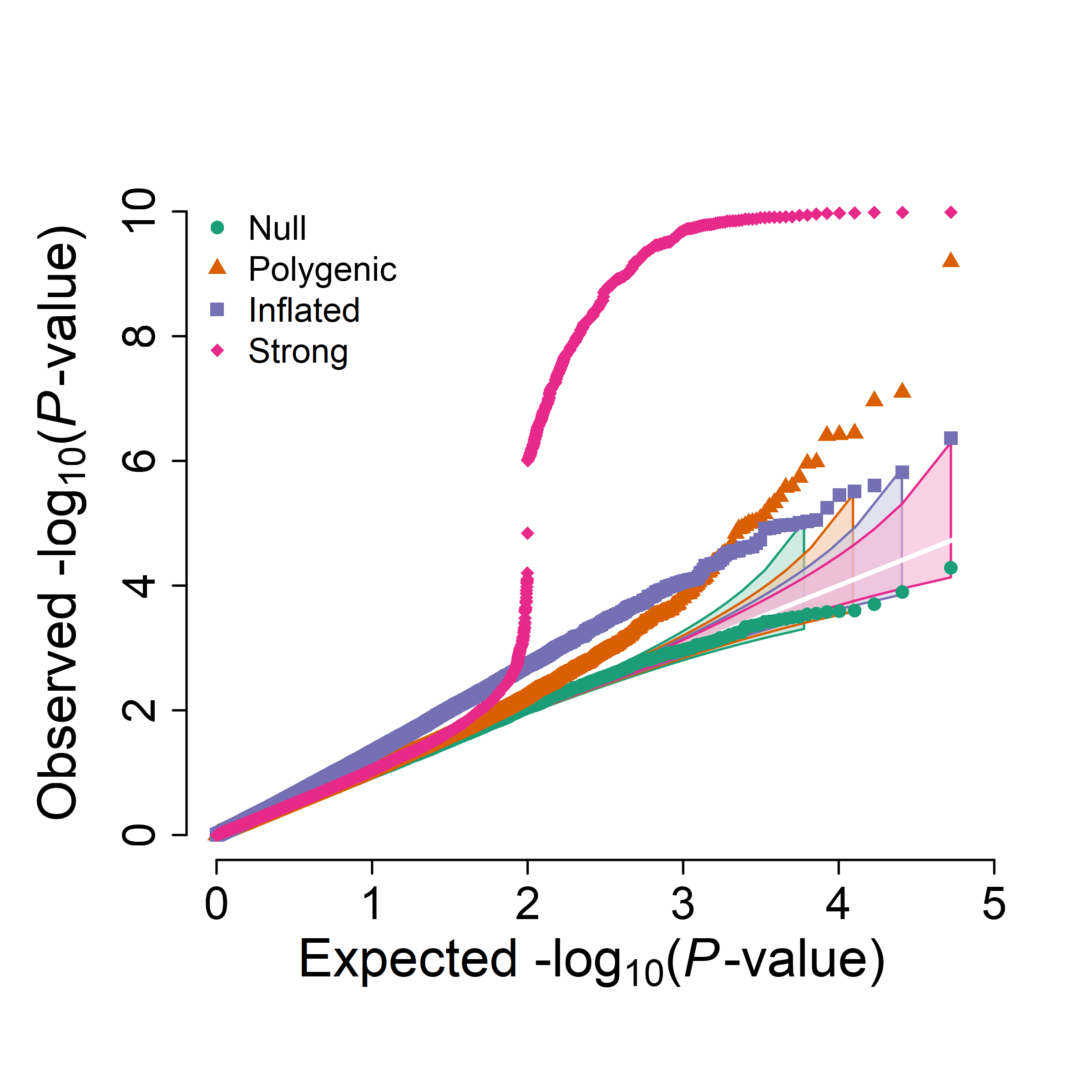
2 multi trait
qqplot_multi <- function(pval_list, ylim=0, lab=1.4, axis=1.2, p_floor=1e-300, cols=NULL, pch=20, cex=0.6,
legend=TRUE, legend_pos="topleft", legend_cex=0.9, show_ci=TRUE, ci_scale=1, ci_alpha=0.6, ci_border=TRUE, diag_col="white", ...) {
    if (!is.list(pval_list)) pval_list=as.list(as.data.frame(pval_list))
    trait = names(pval_list)
    if(is.null(trait) || any(trait == "")){
        trait=paste0("Trait", seq_along(pval_list))
        names(pval_list)=trait
    }

    m = length(pval_list)
    if(m < 1) stop("pval_list must contain at least one trait ! ! !")

    recycle1m = function(x, nm, name){
        if (length(x) == 1) return(rep(x, nm))
        if (length(x) == nm) return(x)
        stop(name, " length must be 1 or ", nm, ".")
    }

    ci_scale = recycle1m(ci_scale , m, "ci_xfrac")
    ci_scale[ci_scale <= 0] = 0.01
    ci_scale[ci_scale > 1]  = 1

    if(is.null(cols)){
        if ("hcl.colors" %in% getNamespaceExports("grDevices")){
            cols = grDevices::hcl.colors(m, palette="Dark 3")
        } else {
            cols = grDevices::rainbow(m)
        }
    }
    cols = recycle1m(cols, m, "cols")
    pch  = recycle1m(pch, m, "pch")

    lighten_col = function(col, amount=0.65, alpha=ci_alpha) {
        rgb  = grDevices::col2rgb(col) / 255
        rgb2 = rgb + (1-rgb) * amount
        grDevices::rgb(rgb2[1,], rgb2[2,], rgb2[3,], alpha=alpha)
    }

    dat=vector("list", m)
    for(i in seq_len(m)){
        p = pval_list[[i]]
        p = p[is.finite(p) & !is.na(p)]
        p = p[p <= 1 & p >= 0]
        if (length(p) == 0) stop("Trait '", trait[i], "' has no valid P in [0,1].")
        p[p == 0] = p_floor

        p2 = sort(p)
        n  = length(p2)
        k  = seq_len(n)
        alpha = 0.05
        lower = qbeta(alpha/2, k, n+1-k)
        upper = qbeta(1 - alpha/2, k, n+1-k)
        expect = (k-0.05) / n
        expect[expect <= 0] = min(expect[expect > 0])

        dat[[i]] = list(x=-log10(expect), y=-log10(p2), y_low=-log10(upper), y_high=-log10(lower), n=n)
    }

    xlim = max(vapply(dat, function(d) max(d$x, na.rm=TRUE), numeric(1))) + 0.1
    ymax = max(vapply(dat, function(d) max(d$y, d$y_high, na.rm=TRUE), numeric(1)))
    if (ylim==0) ylim=ceiling(ymax)

    par(mgp=c(5,1,0))
    plot(NA, xlim=c(0, xlim), ylim=c(0, ylim),
    ylab=expression(paste("Observed", " -", log[10], "(", italic(P), "-value", ")", sep="")),
    xlab=expression(paste("Expected", " -", log[10], "(", italic(P), "-value", ")", sep="")),
    type="n", mgp=c(2,0.5,0), tcl=-0.3, bty="n", cex.lab=lab, cex.axis=axis, ...)

    if (show_ci){
        for(i in seq_len(m)){
            d = dat[[i]]
            o = order(d$x)
            x = d$x[o]
            ylow  = d$y_low[o]
            yhigh = d$y_high[o]
            x_ci  = x * ci_scale[i]
            ylow  = ylow * ci_scale[i]
            yhigh = yhigh * ci_scale[i]

            ci_col = lighten_col(cols[i])
            if (ci_border) {
                border=cols[i]
            } else {
                border=NA
            }
            polygon(c(x_ci, rev(x_ci)), c(ylow, rev(yhigh)), col=ci_col, border=border)
        }
    }
    abline(0, 1, col=diag_col, lwd=2)

    for(i in seq_len(m)){
        d = dat[[i]]
        points(d$x, d$y, pch=pch[i], cex=cex, col=cols[i])
    }

    if (legend){
        legend(legend_pos, legend=trait, col=cols, pch=pch, pt.cex=cex, bty="n", cex=legend_cex)
    }
    invisible(dat)
}
example
set.seed(20260108)

N <- 50000

# 1) 纯零假设(均匀分布)
p_null <- runif(N)

# 2) “多基因/少量真实信号”:97% null + 3% 偏小p
p_poly <- runif(N)
sig_poly <- rbinom(N, 1, 0.03) == 1
p_poly[sig_poly] <- rbeta(sum(sig_poly), shape1 = 0.4, shape2 = 1)  # shape1<1 会产生更多小p

# 3) “膨胀”:|Z|整体偏大(sd>1),p会更偏小但不一定有真实峰
z_inf <- rnorm(N, mean = 0, sd = 1.2)
p_infl <- 2 * pnorm(-abs(z_inf))

# 4) “强信号”:1% 极强关联(生成极小p),并故意加入几个0
p_strong <- runif(N)
idx_strong <- sample.int(N, size = round(0.01 * N))
p_strong[idx_strong] <- 10^(-runif(length(idx_strong), min = 6, max = 10)) # 1e-6 到 1e-30
# p_strong[sample.int(N, 5)] <- 0  # 故意放几个0,测试防 Inf

pvals_list <- list(
  Null      = p_null,
  Polygenic = p_poly,
  Inflated  = p_infl,
  Strong    = p_strong
)

png("qqplot_multi.png", width=2400, height=2400, res=500, type="cairo")
qqplot_multi(
  pvals_list,
  cols = c("#1b9e77", "#d95f02", "#7570b3", "#e7298a"),
  pch  = c(16, 17, 15, 18),
  cex  = c(0.8, 0.8, 0.8, 0.8),
  ci_scale = seq(0.8, 1.0, length.out = 4),
  ci_alpha=0.6)
dev.off()
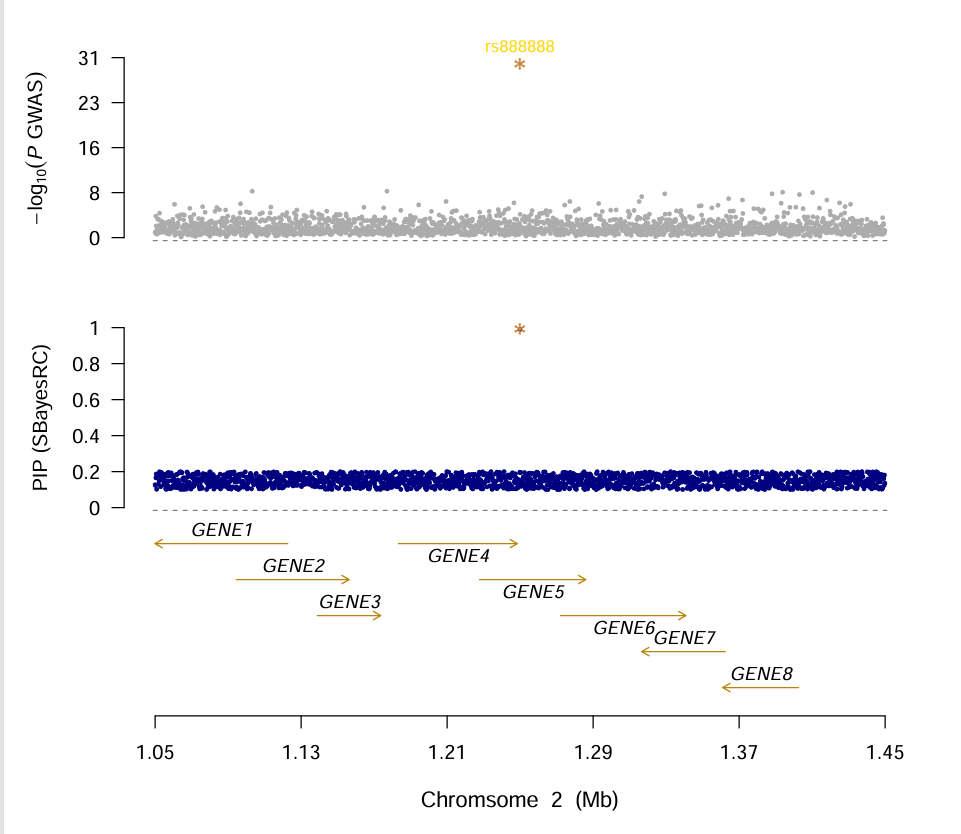
Locus plot for GWFM (genome wide fine mapping)
🧠 When you want draw locus plot of GWFM, follow scripts will meet your require
# ===========================================================================================//
# @Author  :    Loren Shi
# @Time    :    2025/06/05 15:42:36
# @File    :    plot_GWFM.r
# @Mails   :    crazzy_rabbit@163.com
# @line    :    https://github.com/Crazzy-Rabbit
#
# R script to draw regional plot for genome wide fine mapping SNPs.
#
# Part of code are adopted from plot_smr script which provided by SMR
#
# Amendment:
#  2025/06/05
#    1. script completed
#    2. first realeased
#    3. fixed teh bug where the drawn gene was not in the middle of the genelayer when nrowgene=1
#
# Usages:
#     source("plot_GWFM.r")
#     PData <- ReadPvalueFromFiles(gwas="gwas_chrpos.gz", gwfm="gwaf.snpRes", glist="glist_hg19_refseq.txt", windowsize=200000, highlight="rs641221")
#     pdf('gwfm_plot.pdf',width = 8,height = 8)
#     MultiPvalueLocusPlot(data=PData)
#     dev.off()
# ===========================================================================================//
is.installed <- function(mypkg){
    is.element(mypkg, installed.packages()[,1])
}
# check if package "TeachingDemos" is installed
if (!is.installed("TeachingDemos")){
    install.packages("TeachingDemos");
}
library(TeachingDemos)
library(data.table)

# parmeters for plot
genemove=0.01; txt=1.1; cex=1.3; lab=1.1; axis=1; top_cex=1.2;

GeneRowNum = function(GENELIST) {
    BP_THRESH = 0.03; MAX_ROW = 5
    # get the start and end position
    GENELIST = GENELIST[!duplicated(GENELIST$GENE),]
    START1 = as.numeric(GENELIST$GENESTART);
    END1 = as.numeric(GENELIST$GENEEND)
    STRLENGTH = nchar(as.character(GENELIST$GENE))
    MIDPOINT = (START1 + END1)/2
    START2 = MIDPOINT-STRLENGTH/250;
    END2 = MIDPOINT+STRLENGTH/250
    START = cbind(START1, START2);
    END = cbind(END1, END2);
    START = apply(START, 1, min);
    END = apply(END, 1, max)
    GENELIST = data.frame(GENELIST, START, END)
    GENELIST = GENELIST[order(as.numeric(GENELIST$END)),]
    START = as.numeric(GENELIST$START); END = as.numeric(GENELIST$END)
    # get the row index for each gene
    NBUF = dim(GENELIST)[1]
    ROWINDX = rep(1, NBUF)
    ROWEND = as.numeric(rep(0, MAX_ROW))
    MOVEFLAG = as.numeric(rep(0, NBUF))
    if(NBUF>1) {
        for( k in 2 : NBUF ) {
            ITERFLAG=FALSE
            if(START[k] < END[k-1]) {
                INDXBUF=ROWINDX[k-1]+1
            } else INDXBUF = 1
            if(INDXBUF>MAX_ROW) INDXBUF=1;
            REPTIME=0
            repeat{
                if( ROWEND[INDXBUF] > START[k] ) {
                    ITERFLAG=FALSE
                    INDXBUF=INDXBUF+1
                    if(INDXBUF>MAX_ROW) INDXBUF = 1
                } else {
                    ITERFLAG=TRUE
                }
                if(ITERFLAG) break;
                REPTIME = REPTIME+1
                if(REPTIME==MAX_ROW) break;
            }
            ROWINDX[k]=INDXBUF;

            if( (abs(ROWEND[ROWINDX[k]]-START[k]) < BP_THRESH)
            | ((ROWEND[ROWINDX[k]]-START[k])>0) ) {
                MOVEFLAG[k] = 1
                SNBUF = tail(which(ROWINDX[c(1:k)]==ROWINDX[k]), n=2)[1]
                MOVEFLAG[SNBUF] = MOVEFLAG[SNBUF] - 1
            }
            if(ROWEND[ROWINDX[k]]<END[k]) {
                ROWEND[ROWINDX[k]] = END[k]  }
        }
    }
    GENEROW = data.frame(as.character(GENELIST$GENE),
    as.character(GENELIST$ORIENTATION),
    as.numeric(GENELIST$GENESTART),
    as.numeric(GENELIST$GENEEND),
    ROWINDX, MOVEFLAG)
    colnames(GENEROW) = c("GENE", "ORIENTATION", "START", "END", "ROW", "MOVEFLAG")
    return(GENEROW)
}

ReadPvalueFromFiles <- function(gwas, gwfm, glist, windowsize=500000, highlight) {
    gwas1 = fread(gwas)[, .(CHR, POS, SNP, p)]
    colnames(gwas1) = c("CHR", "BP", "SNP", "p")
    gwas1$CHR = as.character(gwas1$CHR)
    gwas2 = fread(gwfm)[, .(Chrom, Position, Name, PIP)]
    colnames(gwas2) = c("CHR", "BP", "SNP", "p")
    gwas2$CHR = as.character(gwas2$CHR)

    snp_gwas1 = gwas1[gwas1$SNP == highlight, ];
    chrom = unique(snp_gwas1$CHR)
    if (nrow(snp_gwas1) == 0) {stop("highlight SNP not found in file1, please check it!")}
    BP1 = snp_gwas1$BP
    start1 = BP1 - windowsize;
    end1 = BP1 + windowsize;
    file1 = gwas1[gwas1$CHR == chrom & gwas1$BP > start1 & gwas1$BP < end1, ]

    snp_gwas2 = gwas2[gwas2$SNP == highlight, ];
    if (nrow(snp_gwas2) == 0) {stop("highlight SNP not found in file2, please check it!")}
    BP2 = snp_gwas2$BP
    start2 = BP2 - windowsize;
    end2 = BP2 + windowsize;
    file2 = gwas2[gwas2$CHR == chrom & gwas2$BP > start2 & gwas2$BP < end2, ]

    start = max(c(start1, start2), na.rm=T) / 1e6;
    end = max(c(end1, end2), na.rm=T) / 1e6;
    glist = fread(glist)
    glist[,2] = glist[,2]/1e6;
    glist[,3] = glist[,3]/1e6;
    colnames(glist) = c("CHR", "GENESTART",  "GENEEND",  "GENE", "ORIENTATION")
    glist = glist[glist$CHR == chrom & glist$GENESTART >= start & glist$GENEEND <= end, ]

    return_lsit = list(file1=file1, file2=file2, SNP=highlight, glist=glist, CHR=chrom)
}


MultiPvalueLocusPlot <- function(data) {
    gwas1 = data$file1;
    gwas2 = data$file2;

    pXY1 = -log10(gwas1$p);
    yMAX = ceiling(max(pXY1, na.rm=T)) + 1;

    pXY2 = gwas2$p;
    yMAX2 = ceiling(max(pXY2, 1, na.rm=T));

    glist = data$glist;
    generow = GeneRowNum(glist);
    num_row = max(as.numeric(generow$ROW));
    offset_map = ceiling(yMAX);
    offset_map = max(offset_map, num_row*2.5);
    offset_pip = yMAX / 2.5;
    dev_axis = 0.1*yMAX;
    if (dev_axis < 1.5) dev_axie=1.5;
    yaxis.min = -offset_map - offset_pip - dev_axis - yMAX;
    yaxis.max = yMAX + ceiling(offset_pip) + 1;
    gwasBP1 = as.numeric(gwas1$BP) / 1e6;
    gwasBP2 = as.numeric(gwas2$BP) / 1e6;
    xmin = min(c(gwasBP1, gwasBP2), na.rm=T) - 0.001;
    xmax = max(c(gwasBP1, gwasBP2), na.rm=T) + 0.001;


    xlab = paste("Chromsome ", data$CHR, " (Mb)")
    #------------------- plot gwas layer ----//
    ylab1 = expression(-log[10] (italic(P) * " GWAS"))
    par(mar=c(5,5,3,2), xpd=TRUE);
    plot(gwasBP1, pXY1, pch=20, xaxt="n", yaxt="n", bty="n", ylim=c(yaxis.min, yaxis.max),
    xlim=c(xmin, xmax), xlab=xlab, ylab="", cex.lab=lab, cex.axis=axis,cex=0.6, col="gray68");
    devbuf1 = yMAX/4;
    xticks = round(seq(xmin, xmax, length.out=6), 2);
    axis(1, at=xticks, lwd=1);
    axis(2, at=seq(0, yMAX, by=devbuf1), labels=round(seq(0, yMAX, devbuf1), 0), las=1, lwd=1);
    mtext(ylab1, side=2, line=3, at=(yMAX*1/2));
    segments(x0=xmin, y0=-0.5, x1=xmax, y1=-0.5, col="grey50", lwd=1, lty=2);

    snp1 = gwas1[SNP == data$SNP, ]
    snpBP1 = snp1$BP / 1e6;
    snpP1 = -log10(snp1$p);

    points(snpBP1, snpP1, pch="*", col="peru", cex=2);
    text(snpBP1, snpP1, labels=snp1$SNP, col="gold", pos=3, cex=0.8, offset=0.5);

    #------------------- plot PIP layer ----//
    ylab2 = "PIP (SBayesRC)"
    axis.start = 0;
    axis.start = axis.start - yMAX - offset_pip - dev_axis;
    pXY2buf = pXY2 / yMAX2*yMAX + axis.start;
    par(new=TRUE);
    plot(gwasBP2, pXY2buf, pch=20, xaxt="n", yaxt="n", bty="n", ylim=c(yaxis.min, yaxis.max),
    xlim=c(xmin, xmax), ylab="", xlab="", cex.lab=lab, cex.axis=axis, cex=0.6, col="navy");
    devbuf2 = yMAX2/5;
    axis(2, at=seq(axis.start, (axis.start+yMAX), yMAX/5), labels=seq(0, yMAX2, devbuf2), las=1, lwd=1);
    mtext(ylab2, side=2, line=3, at=((axis.start + axis.start + yMAX)/2));
    segments(x0=xmin, y0=axis.start-0.5, x1=xmax, y1=axis.start-0.5, col="grey50", lwd=1, lty=2);

    snp2 = gwas2[SNP == data$SNP, ]
    snpBP2 = snp2$BP / 1e6;
    snpP2 = snp2$p / yMAX2*yMAX + axis.start;

    points(snpBP2, snpP2, pch="*", col="peru", cex=2);
    #------------------- plot gene layer ----//
    num_gene = dim(generow)[1]
    dist = offset_map / num_row;
    for (k in 1:num_row) {
        generowbuf = generow[which(as.numeric(generow[, 5]) == k), ]
        xstart = as.numeric(generowbuf[, 3])
        xend = as.numeric(generowbuf[, 4])
        snbuf = which(xend - xstart < 1e-3)
        if (length(snbuf) > 0) {
            xstart[snbuf] = xstart[snbuf] - 0.0025
            xend[snbuf] = xend[snbuf] + 0.0025
        }
        xcenter = (xstart+xend)/2
        xcenter = spread.labs(xcenter, mindiff=0.01, maxiter=1000, min=xmin, max=xmax)
        num_genebuf = dim(generowbuf)[1]
        if (num_row == 1) {
            for (l in 1:num_genebuf) {
                ofs=0.3;
                if (l%%2 == 0) ofs=-0.8;
                ypos = offset_map/2 + yaxis.min - 1;
                code = 1;
                if (generowbuf[l,2] == "+") code=2;
                arrows(x0=xstart[l], y0=ypos, x1=xend[l], y1=ypos, code=code, length=0.07, ylim=c(yaxis.min, yaxis.max),
                col=colors()[75], lwd=1)
                movebuf = as.numeric(generowbuf[l, 6]) * genemove
                text(x=xcenter[l]+movebuf, y=ypos, label=substitute(italic(genename), list(genename=as.character(generowbuf[l,1]))), pos=3, offset=ofs, col="black", cex=0.9)
            }
        } else if (num_row > 1) {
            for (l in 1:num_genebuf) {
                ofs=0.3
                if(l%%2==0) ofs=-0.8
                m = num_row - k
                ypos = m*dist + yaxis.min
                code = 1;
                if (generowbuf[l,2] == "+") code = 2;
                arrows(x0=xstart[l], y0=ypos, x1=xend[l], y1=ypos, code=code, length=0.07, ylim=c(yaxis.min, yaxis.max),
                col=colors()[75], lwd=1)
                movebuf = as.numeric(generowbuf[l,6]) * genemove
                text(x=xcenter[l]+movebuf, y=ypos, label=substitute(italic(genename), list(genename=as.character(generowbuf[l,1]))), pos=3, offset=ofs, col="black", cex=0.9)
            }
        }
    }
}
Example data as follow:
set.seed(123)

n_snps <- 10000
n_genes <- 10

# SNP pos
positions <- as.integer(seq(500000, 2500000, length.out = n_snps))
snp_ids <- paste0("rs", 1000000 + 0:(n_snps - 1))

# highlight SNP(GWAS)
highlight_snp <- data.frame(
  CHR = "2",
  POS = 1250000,
  SNP = "rs888888",
  p = 1e-30
)

# GWAS summary
pvals <- pmax(rbeta(n_snps, 0.4, 5), 1e-8)
gwas_df <- data.frame(
  CHR = rep("2", n_snps),
  POS = positions,
  SNP = snp_ids,
  p = pvals
)

gwas_df <- rbind(gwas_df, highlight_snp)
write.table(gwas_df, file = "sim_gwas_chr2.gz", sep = "\t", row.names = FALSE, quote = FALSE)

# highlight SNP(PIP)
highlight_pip <- data.frame(
  Chrom = "2",
  Position = 1250000,
  Name = "rs888888",
  PIP = 0.99
)

# PIP data, finemapping result
pip_values <- round(runif(n_snps, 0.1, 0.2), 4)
gwfm_df <- data.frame(
  Chrom = rep("2", n_snps),
  Position = positions,
  Name = snp_ids,
  PIP = pip_values
)

gwfm_df <- rbind(gwfm_df, highlight_pip)
write.table(gwfm_df, file = "sim_gwfm.snpRes", sep = "\t", row.names = FALSE, quote = FALSE)

# gene list
gene_starts <- as.integer(seq(1050000, 1450000, length.out = n_genes))
gene_lengths <- sample(30000:80000, n_genes, replace = TRUE)
gene_ends <- gene_starts + gene_lengths

gene_df <- data.frame(
  CHR = rep("2", n_genes),
  GENESTART = gene_starts,
  GENEEND = gene_ends,
  GENE = paste0("GENE", 1:n_genes),
  ORIENTATION = sample(c("+", "-"), n_genes, replace = TRUE)
)

write.table(gene_df, file = "sim_glist_chr2.txt", sep = "\t", row.names = FALSE, quote = FALSE)

# run script
source("plot_GWFM.r")
PData <- ReadPvalueFromFiles(gwas="sim_gwas_chr2.gz", gwfm="sim_gwfm.snpRes", glist="sim_glist_chr2.txt", windowsize=200000, highlight="rs888888")
pdf('gwfm_plot.pdf',width = 8,height = 8)
MultiPvalueLocusPlot(data=PData)
dev.off()
Job submit in supercompute
🧠 When your job number is very large, follow scripts will meet your require 🔁 An ldsc example for large number job submit (if job can split chromosome)
#! /bin/bash
ldsc="/public/home/shilulu/software/ldsc"
bfile="/public/share/wchirdzhq2022/Wulab_share/LDSC/1000G_EUR_Phase3_plink/1000G.EUR.QC"
ldsc_dir="/public/share/wchirdzhq2022/Wulab_share/LDSC"

files=( *.GeneSet )
total=${#files[@]}
batch_size=2
i=0

while [ $i -lt $total ]; do
    batch=()
    job_ids=()

    for ((j=0; j<batch_size && (i + j) < total; j++)); do
        file=("${files[$((i + j))]}")
        annot=$(basename -- "${file}" ".GeneSet")

        cmd1="python ${ldsc}/make_annot.py \
        --gene-set-file ${annot}.GeneSet \
        --gene-coord-file ${ldsc}/Gene_coord.txt \
        --bimfile ${bfile}.{TASK_ID}.bim \
        --windowsize 100000 \
        --annot-file ${annot}.{TASK_ID}.annot.gz"

        sub1=$(qsubshcom "$cmd1" 1 10G ldsc_anot 1:00:00 "-array=1-22")

        cmd2="python ${ldsc}/ldsc.py --l2 \
        --bfile ${bfile}.{TASK_ID} \
        --print-snps ${ldsc_dir}/listHM3.txt \
        --ld-wind-cm 1 \
        --annot ${annot}.{TASK_ID}.annot.gz \
        --thin-annot \
        --out ${annot}.{TASK_ID}"
        jobid=$(qsubshcom "$cmd2" 1 10G ldsc_comp 1:00:00 "-array=1-22 -wait=$sub1")
        echo "🚀 Submitted job $jobid for $annot, waiting for it finish..."

        job_ids+=("$jobid")
    done

    echo "⏳ Waiting for jobs: ${job_ids[*]}"
    times=0
    while true; do
        sleep 30
        all_done=true
        for jid in "${job_ids[@]}"; do
            if squeue -j "$jid" | grep -q "$jid"; then
                all_done=false
                times=$((times + 30))
                echo "⏳ Jobs in batch still running ${times}s..."
                break
            fi
        done

        if $all_done; then
            echo "✅ All jobs in batch completed."
            break
        else
            echo "⏳ Still waiting for some jobs in batch to finish..."
        fi
    done

    i=$((i + batch_size))
done
🔁 An t-test example for large number job submit
#! /bin/bash
THRESHOLD=60
OUTPUT_FILE_THRESHOLD=2400
ARRAY_SIZE=2
JOB_ID_FILE="job_id.txt"
MAX_JOB_ID=100
OUT_DIR="t_stat_blocks_cell"

if [ ! -f "$JOB_ID_FILE" ]; then
    echo 1 > "$JOB_ID_FILE"
fi

cell_type_count=$(wc -l < cell_type.txt)
submit_per_loop=$((ARRAY_SIZE * cell_type_count))

while true; do
    output_file_count=$(ls $OUT_DIR 2>/dev/null | wc -l)
    current_jobs=$(squeue | grep -v "JOBID" | wc -l)

    if [ "$output_file_count" -ge "$OUTPUT_FILE_THRESHOLD" ]; then
        echo "✅ Output file count ($output_file_count) ≥ threshold ($OUTPUT_FILE_THRESHOLD), exit."
        exit 0
    fi

    start_id=$(cat "$JOB_ID_FILE")
    end_id=$((start_id + ARRAY_SIZE -1))

    if [ "$start_id" -gt "$MAX_JOB_ID" ]; then
        echo "🚫 All jobs submitted (up to $MAX_JOB_ID), waiting for output files..."
        sleep 600
        continue
    fi

    if [ "$current_jobs" -lt "$THRESHOLD" ] && [ $((current_jobs + submit_per_loop)) -le "$THRESHOLD" ]; then
        echo "🚀 Submitting jobs: ID range $start_id to $end_id"
        echo "Current jobs: $current_jobs, Will submit: $submit_per_loop"

        while read -r idx cell; do
            qsubshcom "Rscript t-stat.r {TASK_ID} $idx" 10 100G t-stat 10:00:00 "-array=${start_id}-${end_id}"
        done < cell_type.txt

        echo $((end_id + 1)) > "$JOB_ID_FILE"
        sleep $((60 + RANDOM % 30))

    else
        echo "⏳ Current job number too high or not enough capacity, wait and retry"
        sleep 60
    fi
done
Stereo file to scanpy
🧠 When your want transfer stereo-seq file gef to scanpy or seurat, follow scripts will meet your require
conda activate st
# conda create --name st python=3.8
# conda install stereopy -c stereopy -c grst -c numba -c conda-forge -c bioconda

import stereo as st
import scanpy as sc
import warnings
warnings.filterwarnings('ignore')

# read the GEF file
data_path = 'D02567D4.gef'
data = st.io.read_gef(file_path=data_path, bin_size=50)
data.tl.cal_qc()
data.tl.raw_checkpoint()
data.tl.sctransform(res_key='sctransform', inplace=True)

# clustering
data.tl.pca(use_highly_genes=False, n_pcs=30, res_key='pca')
data.tl.neighbors(pca_res_key='pca', n_pcs=30, res_key='neighbors')
data.tl.umap(pca_res_key='pca', neighbors_res_key='neighbors', res_key='umap')
data.tl.leiden(neighbors_res_key='neighbors', res_key='leiden')

# write as stereopy h5ad
st.io.write_h5ad(
        data,
        use_raw=True,
        use_result=True,
        key_record=None,
        output='./D02567D4.h5ad')


data_path = './D02567D4.h5ad'
data = st.io.read_h5ad(
        file_path=data_path,
        flavor='stereopy',
        use_raw=True,
        use_result=True)

#----------------
# transfer to h5ad of scanpy
adata = st.io.stereo_to_anndata(data, flavor='scanpy',output='out.h5ad')
adata.layers["count"] = adata.X.copy()
adata.obs["annotation"] = 'teeth'
adata.write("D02567D4_scanpy.h5ad")
liftover in R
#---- liftover hg38 to hg19
library(rtracklayer)
library(GenomicRanges)

regions = unique(as.character(merged_dt$Gene))
regions_str = strsplit(regions, "-")
bed_df = do.call(rbind, lapply(seq_along(regions), function(i) {
    x = regions_str[[i]]
    chr = x[1]
    start = as.numeric(x[2]) - 1
    end = as.numeric(x[3])
    peak_id = regions[i]
    return(data.frame(chr=chr, start=start, end=end, peak_id=peak_id))
}))

gr <- GRanges(seqnames = bed_df$chr,
            ranges = IRanges(start=bed_df$start, end=bed_df$end),
            peak_id = bed_df$peak_id)
chain <- import.chain("~Wulab/refGenome/hg38/hg38ToHg19.over.chain")

gr_new_list <- liftOver(gr, chain)
gr_new <- unlist(gr_new_list)
gr_clean <- gr_new[elementNROWS(gr_new_list) == 1]
df_clean <- as.data.frame(gr_clean)[, c("seqnames", "start", "end", "peak_id")]
df_clean_unique <- df_clean[!duplicated(df_clean$peak_id), ]
# peak coord file
coords <- df_clean_unique[, c("peak_id", "seqnames", "start", "end")]
colnames(coords) <- c("GENE", "CHR", "START", "END")
coords$CHR <- sub("^chr", "", coords$CHR)
fwrite(coords, "Peak_coord_hg19.txt", sep="\t")
QC for GWAS summary
sums_col_treate <- function(gwas, SNP, A1, A2, freq, P,
                            CHR = NULL, POS = NULL,
                            BETA = NULL, SE = NULL,
                            OR = NULL, Z = NULL, N=NULL) {
    gwas_col = c(
        CHR   =   CHR,
        POS   =   POS,
        SNP   =   SNP,
        A1    =    A1,
        A2    =    A2,
        freq  =  freq,
        b     =  BETA,
        se    =    SE,
        OR    =    OR,
        Z     =     Z,
        p     =     P,
        N     =     N)
    gwas_col = gwas_col[!sapply(gwas_col, is.null)]

    missing_required = setdiff(c("SNP", "A1", "A2", "freq", "p"), names(gwas_col))
    if (length(missing_required) > 0) {
        stop("Missing required columns: ", paste(missing_required, collapse = ", "))
    }
    has_b_se = all(c("b", "se") %in% names(gwas_col))
    has_or   = "OR" %in% names(gwas_col)
    has_z    = "Z" %in% names(gwas_col)
    if (!(has_b_se || has_or || has_z)) {
        stop("Must provide at least one of the following: (BETA + SE), OR, or Z.")
    }

    gwas = gwas[, unname(gwas_col), with=FALSE]
    setnames(gwas, old = unname(gwas_col), new = names(gwas_col))

    valid_p <- !is.na(gwas$p) & gwas$p >= 0 & gwas$p <= 1
    if (has_b_se){
        gwas = gwas[valid_p & !is.na(SNP) & !is.na(b) & !is.na(se) & b != 0, ]
    } else if (has_or){
        gwas = gwas[valid_p & !is.na(SNP) & !is.na(OR), ]
    } else if (has_z){
        gwas = gwas[valid_p & !is.na(SNP) & !is.na(Z), ]
    }

    return(gwas)
}
🧠 How to use it
library(data.table)
gwas = fread("Ever_smoke.fastGWA.gz")
clean = sums_col_treate(gwas, "variant_id", "effect_allele", "other_allele", "effect_allele_frequency", "p_value", BETA="beta", SE="standard_error" N="N")
clean = sums_col_treate(gwas, "SNP", "A1", "A2", "AF1", "P", BETA="BETA", SE="SE", N="N")
clean = clean[, .(SNP, A1, A2, freq, b, se, p, N)]
fwrite(clean, "../cleanGWAS/clean_ever_smoke.fastGWA.gz", sep="\t")