语法函数2-数据处理dplyr包#
读取数据#
在学习R语言过程中,除了使用内置的数据集外,我们更多的需要导入外部数据
数据科学中的文件管理#
把项目所需的文件(代码、数据、图片等),放在一个文件夹里
读取文件
事实上,R语言提供了很多读取数据的函数。下表列出了常见文件格式的读取方法
文件格式 |
R函数 |
|---|---|
txt |
read.table() |
.csv |
read.csv() and readr::read_csv() |
.xls and .xlsx |
readxl::read_excel() and openxlsx::read.xlsx() |
.sav(SPSS files) |
haven::read_sav() and foreign::read.spss() |
.Rdata or rda |
load() |
.rds |
readRDS() and readr::read_rds() |
.dta |
haven::read_dta() and haven::read_stata() |
.sas7bdat(SAS files) |
haven::read_sas() |
Internet |
download.file() |
here宏包#
强大的
here宏包,here()会告诉我们当前所在的目录指向某个文件的路径信息
here宏包的好处还在于,在不同的电脑和文件结构下,代码都能运行
here::here()
here::here("software", "smoove")
d <- read.table(file= "./data/txt_file.txt", header = TRUE)
Warning message in file(file, "rt"):
“无法打开文件'./data/txt_file.txt': 没有那个文件或目录”
Error in file(file, "rt"): 无法打开链结
Traceback:

1. read.table(file = "./data/txt_file.txt", header = TRUE)
2. file(file, "rt")
数据处理#
数据处理的工具
dplyr宏包–tidyverse里的“瑞士军刀”dplyr定义了数据处理的规范语法,其中主要包含以下10个主要的函数mutate(),select(),rename(),filter()summarise(),group_by(),arrange()left_join(),right_join(),full_join()
if_else()case_when()everything()函数count()对给定条件的某列进行计数,
count(x, condition)相当于filter(x,condition) %>% group_by(x) %>% summarise(n=n())
across()对给定的某些列赋予函数计算
across(.cols = everything(), .fns = NULL, ..., .names = NULL)用在
mutate()和summarise()函数里面across()对多列执行相同的函数操作,返回数据框list()列出多个要使用的函数及对应列名
library(dplyr)
载入程辑包:‘dplyr’
The following objects are masked from ‘package:stats’:

    filter, lag
The following objects are masked from ‘package:base’:

    intersect, setdiff, setequal, union
df <- data.frame(
name=c("Alice", "Alice", "Bob", "Bob", "Carol", "Carol"),
type=c("english", "math", "english", "math", "english", "math"),
score=c(80, 60, 70, 69, 80, 90))
df
| name | type | score |
|---|---|---|
| <chr> | <chr> | <dbl> |
| Alice | english | 80 |
| Alice | math | 60 |
| Bob | english | 70 |
| Bob | math | 69 |
| Carol | english | 80 |
| Carol | math | 90 |
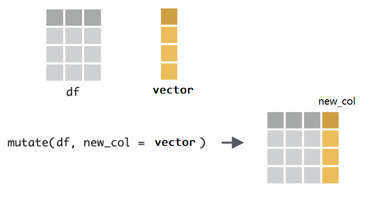
1 新增一列 mutata()#
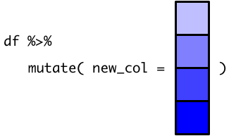
mutate()函数的功能是给数据框新增一列,使用语法为mutate(.data = df, name = value)第一个参数
.data,接受要处理的数据框,比如这里的df第二个参数是
Name-value对, 比如extra = reward,等号左边,是我们为新增的一列取的名字,比如这里的
extra,因为数据框每一列都是要有名字的;等号右边,是打算并入数据框的向量,比如这里的
reward,它是装着学生成绩的向量。注意,向量的长度,要么与数据框的行数等长,比如这里向量长度为6;
要么长度为1,即,新增的这一列所有的值都是一样的(循环补齐机制)。
因为
mutate()函数处理的是数据框,并且固定放置在第一位置上(几乎所有dplyr的函数都是这样要求的),所以这个.data可以偷懒不写,直接写mutate(df, extra = reward)。另外,如果想同时新增多个列,只需要提供多个Name-value对即可
reward <- c(2, 5, 9, 8, 5, 6)
mutate(df, extra=reward)
| name | type | score | extra |
|---|---|---|---|
| <chr> | <chr> | <dbl> | <dbl> |
| Alice | english | 80 | 2 |
| Alice | math | 60 | 5 |
| Bob | english | 70 | 9 |
| Bob | math | 69 | 8 |
| Carol | english | 80 | 5 |
| Carol | math | 90 | 6 |
# 新增多列
mutate(df,
      extra1 = c(2, 5, 9, 8, 5, 6),
      extra2 = c(1, 2, 3, 3, 2, 1),
      extra3 = c(8)
      )
| name | type | score | extra1 | extra2 | extra3 |
|---|---|---|---|---|---|
| <chr> | <chr> | <dbl> | <dbl> | <dbl> | <dbl> |
| Alice | english | 80 | 2 | 1 | 8 |
| Alice | math | 60 | 5 | 2 | 8 |
| Bob | english | 70 | 9 | 3 | 8 |
| Bob | math | 69 | 8 | 3 | 8 |
| Carol | english | 80 | 5 | 2 | 8 |
| Carol | math | 90 | 6 | 1 | 8 |
2 管道 %>%#
Windows系统中可以通过
Ctrl + Shift + M快捷键产生%>%
c(1:10) %>% sum()
这条语句的意思是
f(x)写成x %>% f(),这里向量c(1:10)通过管道操作符%>%,传递到函数sum()的第一个参数位置,即sum(c(1:10))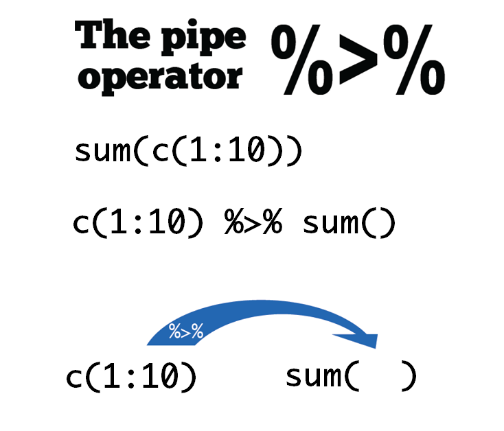
df %>% mutate(extra=reward)
| name | type | score | extra |
|---|---|---|---|
| <chr> | <chr> | <dbl> | <dbl> |
| Alice | english | 80 | 2 |
| Alice | math | 60 | 5 |
| Bob | english | 70 | 9 |
| Bob | math | 69 | 8 |
| Carol | english | 80 | 5 |
| Carol | math | 90 | 6 |
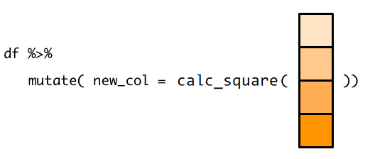
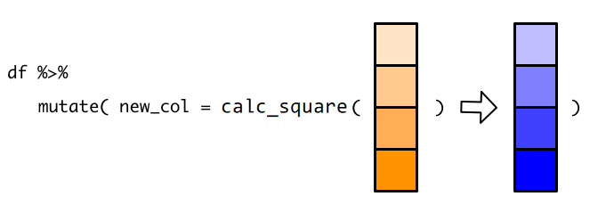
3 向量函数与mutate()#
mutate()函数的本质还是向量函数和向量化操作,只不过是换作在数据框中完成,这样更能形成“数据框进、数据框出”的思维,方便快捷地构思并统计任务在
mutate()中引用数据框的某一列名,实际上是引用了列名对应的整个向量, 所以,这里我们传递score到calc_square(),就是把整个score向量传递给calc_square().几何算符(这里是平方)是向量化的,因此
calc_square()会对输入的score向量,返回一个等长的向量。mutate()拿到这个新的向量后,就在原有数据框中添加新的一列new_col
calc_square <- function(x){
    x^2
}
df %>% mutate(new_col = calc_square(score))
| name | type | score | new_col |
|---|---|---|---|
| <chr> | <chr> | <dbl> | <dbl> |
| Alice | english | 80 | 6400 |
| Alice | math | 60 | 3600 |
| Bob | english | 70 | 4900 |
| Bob | math | 69 | 4761 |
| Carol | english | 80 | 6400 |
| Carol | math | 90 | 8100 |
4 保存为新的数据框#
df_new <- df %>%
  mutate(extra = reward) %>%
  mutate(total = score + extra)
df_new

df_new2 <- df %>%
  mutate(extra = reward,
        total = score + extra)
df_new2
| name | type | score | extra | total |
|---|---|---|---|---|
| <chr> | <chr> | <dbl> | <dbl> | <dbl> |
| Alice | english | 80 | 2 | 82 |
| Alice | math | 60 | 5 | 65 |
| Bob | english | 70 | 9 | 79 |
| Bob | math | 69 | 8 | 77 |
| Carol | english | 80 | 5 | 85 |
| Carol | math | 90 | 6 | 96 |
| name | type | score | extra | total |
|---|---|---|---|---|
| <chr> | <chr> | <dbl> | <dbl> | <dbl> |
| Alice | english | 80 | 2 | 82 |
| Alice | math | 60 | 5 | 65 |
| Bob | english | 70 | 9 | 79 |
| Bob | math | 69 | 8 | 77 |
| Carol | english | 80 | 5 | 85 |
| Carol | math | 90 | 6 | 96 |
5 选取列 select()#
select()顾名思义选择,就是选择数据框的某一列,或者某几列。数据框进数据框出是
dplyr函数的第二个特点删除某列,可以在变量前面加
-或者!,两者的结果是一样的。也可以通过位置索引进行选取
如果要选取数据框的列很多,我们也可以先观察列名的特征,用特定的函数进行选取
df_new %>% select(name, extra)
| name | extra |
|---|---|
| <chr> | <dbl> |
| Alice | 2 |
| Alice | 5 |
| Bob | 9 |
| Bob | 8 |
| Carol | 5 |
| Carol | 6 |
df_new %>% select(-name)
| type | score | extra | total |
|---|---|---|---|
| <chr> | <dbl> | <dbl> | <dbl> |
| english | 80 | 2 | 82 |
| math | 60 | 5 | 65 |
| english | 70 | 9 | 79 |
| math | 69 | 8 | 77 |
| english | 80 | 5 | 85 |
| math | 90 | 6 | 96 |
df_new %>% select(1,2,3)
df_new %>% select(1:3)
| name | type | score |
|---|---|---|
| <chr> | <chr> | <dbl> |
| Alice | english | 80 |
| Alice | math | 60 |
| Bob | english | 70 |
| Bob | math | 69 |
| Carol | english | 80 |
| Carol | math | 90 |
| name | type | score |
|---|---|---|
| <chr> | <chr> | <dbl> |
| Alice | english | 80 |
| Alice | math | 60 |
| Bob | english | 70 |
| Bob | math | 69 |
| Carol | english | 80 |
| Carol | math | 90 |
# 如果要选取数据框的列很多,我们也可以先观察列名的特征,用特定的函数进行选取
df_new %>% select(starts_with("s"))
df_new %>% select(ends_with("e"))
df_new %>% select(contains("score"))  # 列名包含
df_new %>% select(where(is.character)) # 通过变量的类型来选取
df_new %>% select(where(is.numeric))
df_new %>% select(where(is.numeric) & starts_with("t"))
df_new %>% select(!starts_with("s"))
| score |
|---|
| <dbl> |
| 80 |
| 60 |
| 70 |
| 69 |
| 80 |
| 90 |
| name | type | score |
|---|---|---|
| <chr> | <chr> | <dbl> |
| Alice | english | 80 |
| Alice | math | 60 |
| Bob | english | 70 |
| Bob | math | 69 |
| Carol | english | 80 |
| Carol | math | 90 |
| score |
|---|
| <dbl> |
| 80 |
| 60 |
| 70 |
| 69 |
| 80 |
| 90 |
| name | type |
|---|---|
| <chr> | <chr> |
| Alice | english |
| Alice | math |
| Bob | english |
| Bob | math |
| Carol | english |
| Carol | math |
| score | extra | total |
|---|---|---|
| <dbl> | <dbl> | <dbl> |
| 80 | 2 | 82 |
| 60 | 5 | 65 |
| 70 | 9 | 79 |
| 69 | 8 | 77 |
| 80 | 5 | 85 |
| 90 | 6 | 96 |
| total |
|---|
| <dbl> |
| 82 |
| 65 |
| 79 |
| 77 |
| 85 |
| 96 |
| name | type | extra | total |
|---|---|---|---|
| <chr> | <chr> | <dbl> | <dbl> |
| Alice | english | 2 | 82 |
| Alice | math | 5 | 65 |
| Bob | english | 9 | 79 |
| Bob | math | 8 | 77 |
| Carol | english | 5 | 85 |
| Carol | math | 6 | 96 |
6 修改列名 rename()#
用
rename()修改列的名字, 具体方法是rename(.data, new_name = old_name),和mutate()一样,等号左边是新的变量名,右边是已经存在的变量名(这是dplyr函数的第三个特征)
df_new %>%
  select(name, type, total) %>%
  rename(total_score = total)
| name | type | total_score |
|---|---|---|
| <chr> | <chr> | <dbl> |
| Alice | english | 82 |
| Alice | math | 65 |
| Bob | english | 79 |
| Bob | math | 77 |
| Carol | english | 85 |
| Carol | math | 96 |
7 筛选filter()#
前面
select()是列方向的选择,而用filter()函数,我们可以对数据框行方向进行筛选,选出符合特定条件的某些行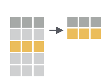
注意,这里
filter()函数不是字面上“过滤掉”的意思,而是保留符合条件的行,也就说keep,不是drop的意思。R提供了其他比较关系的算符:<,>,<=,>=,==(equal),!=(not equal),%in%,is.na()和!is.na().可以限定多个条件进行筛选,支持逻辑运算符
可以配合一些函数使用
filter()中的逻辑运算符
Operator |
Meaning |
|---|---|
|
Equal to |
|
Greater than |
|
Less than |
|
Greater than or equal to |
|
Less than or equal to |
|
Not equal to |
|
in |
|
is a missing value (NA) |
|
is not a missing value |
|
and |
|
or |
df_new %>% filter(score > 70)
| name | type | score | extra | total |
|---|---|---|---|---|
| <chr> | <chr> | <dbl> | <dbl> | <dbl> |
| Alice | english | 80 | 2 | 82 |
| Carol | english | 80 | 5 | 85 |
| Carol | math | 90 | 6 | 96 |
df_new %>% filter(type=="english" & score >= 75)
df_new %>% filter(type=="english", score >= 75)
| name | type | score | extra | total |
|---|---|---|---|---|
| <chr> | <chr> | <dbl> | <dbl> | <dbl> |
| Alice | english | 80 | 2 | 82 |
| Carol | english | 80 | 5 | 85 |
| name | type | score | extra | total |
|---|---|---|---|---|
| <chr> | <chr> | <dbl> | <dbl> | <dbl> |
| Alice | english | 80 | 2 | 82 |
| Carol | english | 80 | 5 | 85 |
df_new %>% filter(score == max(score))
| name | type | score | extra | total |
|---|---|---|---|---|
| <chr> | <chr> | <dbl> | <dbl> | <dbl> |
| Carol | math | 90 | 6 | 96 |
8 统计汇总summarise()#
summarise()函数非常强大,主要用于统计汇总,往往与其他函数配合使用
df_new %>% summarise(mean_score = mean(score))
df_new %>% summarise(sd_score = sd(score))
| mean_score |
|---|
| <dbl> |
| 74.83333 |
| sd_score |
|---|
| <dbl> |
| 10.59088 |
df_new %>% summarise(
  mean_score = mean(score),
  median_score = median(score),
  n = n(),
  sum = sum(score))
| mean_score | median_score | n | sum |
|---|---|---|---|
| <dbl> | <dbl> | <int> | <dbl> |
| 74.83333 | 75 | 6 | 449 |
9 分组统计 group_by()#
实际运用中,
summarise()函数往往配合group_by()一起使用,即,先分组再统计
df_new %>%
  group_by(name) %>%
  summarise(
    mean_score = mean(total),
    sd_score = sd(total))
| name | mean_score | sd_score |
|---|---|---|
| <chr> | <dbl> | <dbl> |
| Alice | 73.5 | 12.020815 |
| Bob | 78.0 | 1.414214 |
| Carol | 90.5 | 7.778175 |
10 排序 arrange()#
arrange()就是按照某个变量进行排序,默认为从小到大排序在要排序的变量前加上
-可改成从大到小排序使用
desc()函数也可实现从大到小排序也可对多个变量依次排序
df_new %>% arrange(total)
df_new %>% arrange(-total)
df_new %>% arrange(desc(total))
| name | type | score | extra | total |
|---|---|---|---|---|
| <chr> | <chr> | <dbl> | <dbl> | <dbl> |
| Alice | math | 60 | 5 | 65 |
| Bob | math | 69 | 8 | 77 |
| Bob | english | 70 | 9 | 79 |
| Alice | english | 80 | 2 | 82 |
| Carol | english | 80 | 5 | 85 |
| Carol | math | 90 | 6 | 96 |
| name | type | score | extra | total |
|---|---|---|---|---|
| <chr> | <chr> | <dbl> | <dbl> | <dbl> |
| Carol | math | 90 | 6 | 96 |
| Carol | english | 80 | 5 | 85 |
| Alice | english | 80 | 2 | 82 |
| Bob | english | 70 | 9 | 79 |
| Bob | math | 69 | 8 | 77 |
| Alice | math | 60 | 5 | 65 |
| name | type | score | extra | total |
|---|---|---|---|---|
| <chr> | <chr> | <dbl> | <dbl> | <dbl> |
| Carol | math | 90 | 6 | 96 |
| Carol | english | 80 | 5 | 85 |
| Alice | english | 80 | 2 | 82 |
| Bob | english | 70 | 9 | 79 |
| Bob | math | 69 | 8 | 77 |
| Alice | math | 60 | 5 | 65 |
df_new %>%
  arrange(type, desc(total))
| name | type | score | extra | total |
|---|---|---|---|---|
| <chr> | <chr> | <dbl> | <dbl> | <dbl> |
| Carol | english | 80 | 5 | 85 |
| Alice | english | 80 | 2 | 82 |
| Bob | english | 70 | 9 | 79 |
| Carol | math | 90 | 6 | 96 |
| Bob | math | 69 | 8 | 77 |
| Alice | math | 60 | 5 | 65 |
11 左联结 left_join()#
实际操作中,会遇到数据框合并的情形
left_join(df1, df2, by = "name"),by指定通过哪一列进行合并,合并按照df1进行
df1 <- df_new %>%
  group_by(name) %>%
  summarise(
    mean_score = mean(total)
  )
df1

df2 <- tibble(
       name = c("Alice", "Bob", "Dave"),
       age =  c(12, 13, 14)
)
df2
# 使用 left_join()函数 把两个数据框df1和df2合并连接在一起
left_join(df1, df2, by = "name")
df1 %>% left_join(df2, by = "name")
| name | mean_score |
|---|---|
| <chr> | <dbl> |
| Alice | 73.5 |
| Bob | 78.0 |
| Carol | 90.5 |
| name | age |
|---|---|
| <chr> | <dbl> |
| Alice | 12 |
| Bob | 13 |
| Dave | 14 |
| name | mean_score | age |
|---|---|---|
| <chr> | <dbl> | <dbl> |
| Alice | 73.5 | 12 |
| Bob | 78.0 | 13 |
| Carol | 90.5 | NA |
| name | mean_score | age |
|---|---|---|
| <chr> | <dbl> | <dbl> |
| Alice | 73.5 | 12 |
| Bob | 78.0 | 13 |
| Carol | 90.5 | NA |
12 右联结 right_join()#
right_join(df1, df2, by = "name"),by指定通过哪一列进行合并,合并按照df2进行,没有对应信息计为NA
df1 %>% right_join(df2, by = "name")
| name | mean_score | age |
|---|---|---|
| <chr> | <dbl> | <dbl> |
| Alice | 73.5 | 12 |
| Bob | 78.0 | 13 |
| Dave | NA | 14 |
13 满联结 full_join()#
有时候,我们不想丢失项,可以使用
full_join(),该函数确保条目是完整的,信息缺失的地方为NA
df1 %>% full_join(df2, by = "name")
| name | mean_score | age |
|---|---|---|
| <chr> | <dbl> | <dbl> |
| Alice | 73.5 | 12 |
| Bob | 78.0 | 13 |
| Carol | 90.5 | NA |
| Dave | NA | 14 |
14 内联结inner_join()#
只保留
name条目相同地记录
df1 %>% inner_join(df2, by = "name")
| name | mean_score | age |
|---|---|---|
| <chr> | <dbl> | <dbl> |
| Alice | 73.5 | 12 |
| Bob | 78.0 | 13 |
15 筛选联结 semi_join(x,y) anti_join(x,y)#
筛选联结,有两个
semi_join(x, y)和anti_join(x, y),函数不改变数据框
x的变量的数量,主要影响的是x的观测,也就说会剔除一些行,其功能类似filter()半联结
semi_join(x, y),保留name与y的name相一致的所有行,可以看作对x的筛选反联结
anti_join(x, y),丢弃name与y的name相一致的所有行
df1 %>% semi_join(df2, by="name")
df1 %>% filter(
  name %in% df2$name)
| name | mean_score |
|---|---|
| <chr> | <dbl> |
| Alice | 73.5 |
| Bob | 78.0 |
| name | mean_score |
|---|---|
| <chr> | <dbl> |
| Alice | 73.5 |
| Bob | 78.0 |
df1 %>% anti_join(df2, by="name")
df1 %>% filter(
  ! name %in% df2$name)
| name | mean_score |
|---|---|
| <chr> | <dbl> |
| Carol | 90.5 |
| name | mean_score |
|---|---|
| <chr> | <dbl> |
| Carol | 90.5 |
df %>%
  group_by(name) %>%
  summarise(mean_score = mean(score))

df %>%
  group_by(name) %>%
  mutate(mean_score = mean(score))
| name | mean_score |
|---|---|
| <chr> | <dbl> |
| Alice | 70.0 |
| Bob | 69.5 |
| Carol | 85.0 |
| name | type | score | mean_score |
|---|---|---|---|
| <chr> | <chr> | <dbl> | <dbl> |
| Alice | english | 80 | 70.0 |
| Alice | math | 60 | 70.0 |
| Bob | english | 70 | 69.5 |
| Bob | math | 69 | 69.5 |
| Carol | english | 80 | 85.0 |
| Carol | math | 90 | 85.0 |
dplyr进阶#
导入数据#
library(tidyverse)
library(palmerpenguins)
── Attaching core tidyverse packages ───────────────────────────────────────────────────────────────────────────────────────────────────────────────────────── tidyverse 2.0.0 ──
✔ forcats   1.0.0     ✔ readr     2.1.5
✔ ggplot2   3.5.0     ✔ stringr   1.5.1
✔ lubridate 1.9.3     ✔ tibble    3.2.1
✔ purrr     1.0.2     ✔ tidyr     1.3.1
── Conflicts ─────────────────────────────────────────────────────────────────────────────────────────────────────────────────────────────────────────── tidyverse_conflicts() ──
✖ dplyr::filter() masks stats::filter()
✖ dplyr::lag()    masks stats::lag()
ℹ Use the conflicted package (<http://conflicted.r-lib.org/>) to force all conflicts to become errors
penguins <- penguins %>% drop_na()
penguins %>% select(bill_length_mm, bill_depth_mm)
penguins %>% select(starts_with("bill_"))
| bill_length_mm | bill_depth_mm |
|---|---|
| <dbl> | <dbl> |
| 39.1 | 18.7 |
| 39.5 | 17.4 |
| 40.3 | 18.0 |
| 36.7 | 19.3 |
| 39.3 | 20.6 |
| 38.9 | 17.8 |
| 39.2 | 19.6 |
| 41.1 | 17.6 |
| 38.6 | 21.2 |
| 34.6 | 21.1 |
| 36.6 | 17.8 |
| 38.7 | 19.0 |
| 42.5 | 20.7 |
| 34.4 | 18.4 |
| 46.0 | 21.5 |
| 37.8 | 18.3 |
| 37.7 | 18.7 |
| 35.9 | 19.2 |
| 38.2 | 18.1 |
| 38.8 | 17.2 |
| 35.3 | 18.9 |
| 40.6 | 18.6 |
| 40.5 | 17.9 |
| 37.9 | 18.6 |
| 40.5 | 18.9 |
| 39.5 | 16.7 |
| 37.2 | 18.1 |
| 39.5 | 17.8 |
| 40.9 | 18.9 |
| 36.4 | 17.0 |
| ⋮ | ⋮ |
| 46.9 | 16.6 |
| 53.5 | 19.9 |
| 49.0 | 19.5 |
| 46.2 | 17.5 |
| 50.9 | 19.1 |
| 45.5 | 17.0 |
| 50.9 | 17.9 |
| 50.8 | 18.5 |
| 50.1 | 17.9 |
| 49.0 | 19.6 |
| 51.5 | 18.7 |
| 49.8 | 17.3 |
| 48.1 | 16.4 |
| 51.4 | 19.0 |
| 45.7 | 17.3 |
| 50.7 | 19.7 |
| 42.5 | 17.3 |
| 52.2 | 18.8 |
| 45.2 | 16.6 |
| 49.3 | 19.9 |
| 50.2 | 18.8 |
| 45.6 | 19.4 |
| 51.9 | 19.5 |
| 46.8 | 16.5 |
| 45.7 | 17.0 |
| 55.8 | 19.8 |
| 43.5 | 18.1 |
| 49.6 | 18.2 |
| 50.8 | 19.0 |
| 50.2 | 18.7 |
penguins %>% select(where(is.numeric))
penguins %>% select(!where(is.character))
| bill_length_mm | bill_depth_mm | flipper_length_mm | body_mass_g | year |
|---|---|---|---|---|
| <dbl> | <dbl> | <int> | <int> | <int> |
| 39.1 | 18.7 | 181 | 3750 | 2007 |
| 39.5 | 17.4 | 186 | 3800 | 2007 |
| 40.3 | 18.0 | 195 | 3250 | 2007 |
| 36.7 | 19.3 | 193 | 3450 | 2007 |
| 39.3 | 20.6 | 190 | 3650 | 2007 |
| 38.9 | 17.8 | 181 | 3625 | 2007 |
| 39.2 | 19.6 | 195 | 4675 | 2007 |
| 41.1 | 17.6 | 182 | 3200 | 2007 |
| 38.6 | 21.2 | 191 | 3800 | 2007 |
| 34.6 | 21.1 | 198 | 4400 | 2007 |
| 36.6 | 17.8 | 185 | 3700 | 2007 |
| 38.7 | 19.0 | 195 | 3450 | 2007 |
| 42.5 | 20.7 | 197 | 4500 | 2007 |
| 34.4 | 18.4 | 184 | 3325 | 2007 |
| 46.0 | 21.5 | 194 | 4200 | 2007 |
| 37.8 | 18.3 | 174 | 3400 | 2007 |
| 37.7 | 18.7 | 180 | 3600 | 2007 |
| 35.9 | 19.2 | 189 | 3800 | 2007 |
| 38.2 | 18.1 | 185 | 3950 | 2007 |
| 38.8 | 17.2 | 180 | 3800 | 2007 |
| 35.3 | 18.9 | 187 | 3800 | 2007 |
| 40.6 | 18.6 | 183 | 3550 | 2007 |
| 40.5 | 17.9 | 187 | 3200 | 2007 |
| 37.9 | 18.6 | 172 | 3150 | 2007 |
| 40.5 | 18.9 | 180 | 3950 | 2007 |
| 39.5 | 16.7 | 178 | 3250 | 2007 |
| 37.2 | 18.1 | 178 | 3900 | 2007 |
| 39.5 | 17.8 | 188 | 3300 | 2007 |
| 40.9 | 18.9 | 184 | 3900 | 2007 |
| 36.4 | 17.0 | 195 | 3325 | 2007 |
| ⋮ | ⋮ | ⋮ | ⋮ | ⋮ |
| 46.9 | 16.6 | 192 | 2700 | 2008 |
| 53.5 | 19.9 | 205 | 4500 | 2008 |
| 49.0 | 19.5 | 210 | 3950 | 2008 |
| 46.2 | 17.5 | 187 | 3650 | 2008 |
| 50.9 | 19.1 | 196 | 3550 | 2008 |
| 45.5 | 17.0 | 196 | 3500 | 2008 |
| 50.9 | 17.9 | 196 | 3675 | 2009 |
| 50.8 | 18.5 | 201 | 4450 | 2009 |
| 50.1 | 17.9 | 190 | 3400 | 2009 |
| 49.0 | 19.6 | 212 | 4300 | 2009 |
| 51.5 | 18.7 | 187 | 3250 | 2009 |
| 49.8 | 17.3 | 198 | 3675 | 2009 |
| 48.1 | 16.4 | 199 | 3325 | 2009 |
| 51.4 | 19.0 | 201 | 3950 | 2009 |
| 45.7 | 17.3 | 193 | 3600 | 2009 |
| 50.7 | 19.7 | 203 | 4050 | 2009 |
| 42.5 | 17.3 | 187 | 3350 | 2009 |
| 52.2 | 18.8 | 197 | 3450 | 2009 |
| 45.2 | 16.6 | 191 | 3250 | 2009 |
| 49.3 | 19.9 | 203 | 4050 | 2009 |
| 50.2 | 18.8 | 202 | 3800 | 2009 |
| 45.6 | 19.4 | 194 | 3525 | 2009 |
| 51.9 | 19.5 | 206 | 3950 | 2009 |
| 46.8 | 16.5 | 189 | 3650 | 2009 |
| 45.7 | 17.0 | 195 | 3650 | 2009 |
| 55.8 | 19.8 | 207 | 4000 | 2009 |
| 43.5 | 18.1 | 202 | 3400 | 2009 |
| 49.6 | 18.2 | 193 | 3775 | 2009 |
| 50.8 | 19.0 | 210 | 4100 | 2009 |
| 50.2 | 18.7 | 198 | 3775 | 2009 |
| species | island | bill_length_mm | bill_depth_mm | flipper_length_mm | body_mass_g | sex | year |
|---|---|---|---|---|---|---|---|
| <fct> | <fct> | <dbl> | <dbl> | <int> | <int> | <fct> | <int> |
| Adelie | Torgersen | 39.1 | 18.7 | 181 | 3750 | male | 2007 |
| Adelie | Torgersen | 39.5 | 17.4 | 186 | 3800 | female | 2007 |
| Adelie | Torgersen | 40.3 | 18.0 | 195 | 3250 | female | 2007 |
| Adelie | Torgersen | 36.7 | 19.3 | 193 | 3450 | female | 2007 |
| Adelie | Torgersen | 39.3 | 20.6 | 190 | 3650 | male | 2007 |
| Adelie | Torgersen | 38.9 | 17.8 | 181 | 3625 | female | 2007 |
| Adelie | Torgersen | 39.2 | 19.6 | 195 | 4675 | male | 2007 |
| Adelie | Torgersen | 41.1 | 17.6 | 182 | 3200 | female | 2007 |
| Adelie | Torgersen | 38.6 | 21.2 | 191 | 3800 | male | 2007 |
| Adelie | Torgersen | 34.6 | 21.1 | 198 | 4400 | male | 2007 |
| Adelie | Torgersen | 36.6 | 17.8 | 185 | 3700 | female | 2007 |
| Adelie | Torgersen | 38.7 | 19.0 | 195 | 3450 | female | 2007 |
| Adelie | Torgersen | 42.5 | 20.7 | 197 | 4500 | male | 2007 |
| Adelie | Torgersen | 34.4 | 18.4 | 184 | 3325 | female | 2007 |
| Adelie | Torgersen | 46.0 | 21.5 | 194 | 4200 | male | 2007 |
| Adelie | Biscoe | 37.8 | 18.3 | 174 | 3400 | female | 2007 |
| Adelie | Biscoe | 37.7 | 18.7 | 180 | 3600 | male | 2007 |
| Adelie | Biscoe | 35.9 | 19.2 | 189 | 3800 | female | 2007 |
| Adelie | Biscoe | 38.2 | 18.1 | 185 | 3950 | male | 2007 |
| Adelie | Biscoe | 38.8 | 17.2 | 180 | 3800 | male | 2007 |
| Adelie | Biscoe | 35.3 | 18.9 | 187 | 3800 | female | 2007 |
| Adelie | Biscoe | 40.6 | 18.6 | 183 | 3550 | male | 2007 |
| Adelie | Biscoe | 40.5 | 17.9 | 187 | 3200 | female | 2007 |
| Adelie | Biscoe | 37.9 | 18.6 | 172 | 3150 | female | 2007 |
| Adelie | Biscoe | 40.5 | 18.9 | 180 | 3950 | male | 2007 |
| Adelie | Dream | 39.5 | 16.7 | 178 | 3250 | female | 2007 |
| Adelie | Dream | 37.2 | 18.1 | 178 | 3900 | male | 2007 |
| Adelie | Dream | 39.5 | 17.8 | 188 | 3300 | female | 2007 |
| Adelie | Dream | 40.9 | 18.9 | 184 | 3900 | male | 2007 |
| Adelie | Dream | 36.4 | 17.0 | 195 | 3325 | female | 2007 |
| ⋮ | ⋮ | ⋮ | ⋮ | ⋮ | ⋮ | ⋮ | ⋮ |
| Chinstrap | Dream | 46.9 | 16.6 | 192 | 2700 | female | 2008 |
| Chinstrap | Dream | 53.5 | 19.9 | 205 | 4500 | male | 2008 |
| Chinstrap | Dream | 49.0 | 19.5 | 210 | 3950 | male | 2008 |
| Chinstrap | Dream | 46.2 | 17.5 | 187 | 3650 | female | 2008 |
| Chinstrap | Dream | 50.9 | 19.1 | 196 | 3550 | male | 2008 |
| Chinstrap | Dream | 45.5 | 17.0 | 196 | 3500 | female | 2008 |
| Chinstrap | Dream | 50.9 | 17.9 | 196 | 3675 | female | 2009 |
| Chinstrap | Dream | 50.8 | 18.5 | 201 | 4450 | male | 2009 |
| Chinstrap | Dream | 50.1 | 17.9 | 190 | 3400 | female | 2009 |
| Chinstrap | Dream | 49.0 | 19.6 | 212 | 4300 | male | 2009 |
| Chinstrap | Dream | 51.5 | 18.7 | 187 | 3250 | male | 2009 |
| Chinstrap | Dream | 49.8 | 17.3 | 198 | 3675 | female | 2009 |
| Chinstrap | Dream | 48.1 | 16.4 | 199 | 3325 | female | 2009 |
| Chinstrap | Dream | 51.4 | 19.0 | 201 | 3950 | male | 2009 |
| Chinstrap | Dream | 45.7 | 17.3 | 193 | 3600 | female | 2009 |
| Chinstrap | Dream | 50.7 | 19.7 | 203 | 4050 | male | 2009 |
| Chinstrap | Dream | 42.5 | 17.3 | 187 | 3350 | female | 2009 |
| Chinstrap | Dream | 52.2 | 18.8 | 197 | 3450 | male | 2009 |
| Chinstrap | Dream | 45.2 | 16.6 | 191 | 3250 | female | 2009 |
| Chinstrap | Dream | 49.3 | 19.9 | 203 | 4050 | male | 2009 |
| Chinstrap | Dream | 50.2 | 18.8 | 202 | 3800 | male | 2009 |
| Chinstrap | Dream | 45.6 | 19.4 | 194 | 3525 | female | 2009 |
| Chinstrap | Dream | 51.9 | 19.5 | 206 | 3950 | male | 2009 |
| Chinstrap | Dream | 46.8 | 16.5 | 189 | 3650 | female | 2009 |
| Chinstrap | Dream | 45.7 | 17.0 | 195 | 3650 | female | 2009 |
| Chinstrap | Dream | 55.8 | 19.8 | 207 | 4000 | male | 2009 |
| Chinstrap | Dream | 43.5 | 18.1 | 202 | 3400 | female | 2009 |
| Chinstrap | Dream | 49.6 | 18.2 | 193 | 3775 | male | 2009 |
| Chinstrap | Dream | 50.8 | 19.0 | 210 | 4100 | male | 2009 |
| Chinstrap | Dream | 50.2 | 18.7 | 198 | 3775 | female | 2009 |
# 多种组合选择
penguins %>% select(species, starts_with("bill_"))
| species | bill_length_mm | bill_depth_mm |
|---|---|---|
| <fct> | <dbl> | <dbl> |
| Adelie | 39.1 | 18.7 |
| Adelie | 39.5 | 17.4 |
| Adelie | 40.3 | 18.0 |
| Adelie | 36.7 | 19.3 |
| Adelie | 39.3 | 20.6 |
| Adelie | 38.9 | 17.8 |
| Adelie | 39.2 | 19.6 |
| Adelie | 41.1 | 17.6 |
| Adelie | 38.6 | 21.2 |
| Adelie | 34.6 | 21.1 |
| Adelie | 36.6 | 17.8 |
| Adelie | 38.7 | 19.0 |
| Adelie | 42.5 | 20.7 |
| Adelie | 34.4 | 18.4 |
| Adelie | 46.0 | 21.5 |
| Adelie | 37.8 | 18.3 |
| Adelie | 37.7 | 18.7 |
| Adelie | 35.9 | 19.2 |
| Adelie | 38.2 | 18.1 |
| Adelie | 38.8 | 17.2 |
| Adelie | 35.3 | 18.9 |
| Adelie | 40.6 | 18.6 |
| Adelie | 40.5 | 17.9 |
| Adelie | 37.9 | 18.6 |
| Adelie | 40.5 | 18.9 |
| Adelie | 39.5 | 16.7 |
| Adelie | 37.2 | 18.1 |
| Adelie | 39.5 | 17.8 |
| Adelie | 40.9 | 18.9 |
| Adelie | 36.4 | 17.0 |
| ⋮ | ⋮ | ⋮ |
| Chinstrap | 46.9 | 16.6 |
| Chinstrap | 53.5 | 19.9 |
| Chinstrap | 49.0 | 19.5 |
| Chinstrap | 46.2 | 17.5 |
| Chinstrap | 50.9 | 19.1 |
| Chinstrap | 45.5 | 17.0 |
| Chinstrap | 50.9 | 17.9 |
| Chinstrap | 50.8 | 18.5 |
| Chinstrap | 50.1 | 17.9 |
| Chinstrap | 49.0 | 19.6 |
| Chinstrap | 51.5 | 18.7 |
| Chinstrap | 49.8 | 17.3 |
| Chinstrap | 48.1 | 16.4 |
| Chinstrap | 51.4 | 19.0 |
| Chinstrap | 45.7 | 17.3 |
| Chinstrap | 50.7 | 19.7 |
| Chinstrap | 42.5 | 17.3 |
| Chinstrap | 52.2 | 18.8 |
| Chinstrap | 45.2 | 16.6 |
| Chinstrap | 49.3 | 19.9 |
| Chinstrap | 50.2 | 18.8 |
| Chinstrap | 45.6 | 19.4 |
| Chinstrap | 51.9 | 19.5 |
| Chinstrap | 46.8 | 16.5 |
| Chinstrap | 45.7 | 17.0 |
| Chinstrap | 55.8 | 19.8 |
| Chinstrap | 43.5 | 18.1 |
| Chinstrap | 49.6 | 18.2 |
| Chinstrap | 50.8 | 19.0 |
| Chinstrap | 50.2 | 18.7 |
## 返回向量
my_tibble[["x"]]
my_tibble$x
my_tibble %>% pull(x)
Error in eval(expr, envir, enclos): 找不到对象'my_tibble'
Traceback:
# 返回数据框
my_tibble["x"]
my_tibble %>% select(x)
Error in eval(expr, envir, enclos): 找不到对象'my_tibble'
Traceback:
tb <- tibble(
  x = 1:5,
  y = 0,
  z = 5:1,
  w = 0
)
tb
| x | y | z | w |
|---|---|---|---|
| <int> | <dbl> | <int> | <dbl> |
| 1 | 0 | 5 | 0 |
| 2 | 0 | 4 | 0 |
| 3 | 0 | 3 | 0 |
| 4 | 0 | 2 | 0 |
| 5 | 0 | 1 | 0 |
myfun <- function(x) sum(x) == 0

tb %>% select(where(myfun))

tb %>% select(where(~sum(.x) == 0))
| y | w |
|---|---|
| <dbl> | <dbl> |
| 0 | 0 |
| 0 | 0 |
| 0 | 0 |
| 0 | 0 |
| 0 | 0 |
| y | w |
|---|---|
| <dbl> | <dbl> |
| 0 | 0 |
| 0 | 0 |
| 0 | 0 |
| 0 | 0 |
| 0 | 0 |
df <- tibble(
  x = c(NA, NA, NA),
  y = c(2, 3, NA),
  z = c(NA, 5, NA)
)
df

df %>% select(where(~ !all(is.na(.x))))
df %>% filter(if_any(everything(), ~ !is.na(.x)))
| x | y | z |
|---|---|---|
| <lgl> | <dbl> | <dbl> |
| NA | 2 | NA |
| NA | 3 | 5 |
| NA | NA | NA |
| y | z |
|---|---|
| <dbl> | <dbl> |
| 2 | NA |
| 3 | 5 |
| NA | NA |
| x | y | z |
|---|---|---|
| <lgl> | <dbl> | <dbl> |
| NA | 2 | NA |
| NA | 3 | 5 |
penguins %>% filter(species %in% c("Adelie", "Gentoo"))
penguins %>% filter(species == "Adelie" & bill_length_mm > 40)
| species | island | bill_length_mm | bill_depth_mm | flipper_length_mm | body_mass_g | sex | year |
|---|---|---|---|---|---|---|---|
| <fct> | <fct> | <dbl> | <dbl> | <int> | <int> | <fct> | <int> |
| Adelie | Torgersen | 39.1 | 18.7 | 181 | 3750 | male | 2007 |
| Adelie | Torgersen | 39.5 | 17.4 | 186 | 3800 | female | 2007 |
| Adelie | Torgersen | 40.3 | 18.0 | 195 | 3250 | female | 2007 |
| Adelie | Torgersen | 36.7 | 19.3 | 193 | 3450 | female | 2007 |
| Adelie | Torgersen | 39.3 | 20.6 | 190 | 3650 | male | 2007 |
| Adelie | Torgersen | 38.9 | 17.8 | 181 | 3625 | female | 2007 |
| Adelie | Torgersen | 39.2 | 19.6 | 195 | 4675 | male | 2007 |
| Adelie | Torgersen | 41.1 | 17.6 | 182 | 3200 | female | 2007 |
| Adelie | Torgersen | 38.6 | 21.2 | 191 | 3800 | male | 2007 |
| Adelie | Torgersen | 34.6 | 21.1 | 198 | 4400 | male | 2007 |
| Adelie | Torgersen | 36.6 | 17.8 | 185 | 3700 | female | 2007 |
| Adelie | Torgersen | 38.7 | 19.0 | 195 | 3450 | female | 2007 |
| Adelie | Torgersen | 42.5 | 20.7 | 197 | 4500 | male | 2007 |
| Adelie | Torgersen | 34.4 | 18.4 | 184 | 3325 | female | 2007 |
| Adelie | Torgersen | 46.0 | 21.5 | 194 | 4200 | male | 2007 |
| Adelie | Biscoe | 37.8 | 18.3 | 174 | 3400 | female | 2007 |
| Adelie | Biscoe | 37.7 | 18.7 | 180 | 3600 | male | 2007 |
| Adelie | Biscoe | 35.9 | 19.2 | 189 | 3800 | female | 2007 |
| Adelie | Biscoe | 38.2 | 18.1 | 185 | 3950 | male | 2007 |
| Adelie | Biscoe | 38.8 | 17.2 | 180 | 3800 | male | 2007 |
| Adelie | Biscoe | 35.3 | 18.9 | 187 | 3800 | female | 2007 |
| Adelie | Biscoe | 40.6 | 18.6 | 183 | 3550 | male | 2007 |
| Adelie | Biscoe | 40.5 | 17.9 | 187 | 3200 | female | 2007 |
| Adelie | Biscoe | 37.9 | 18.6 | 172 | 3150 | female | 2007 |
| Adelie | Biscoe | 40.5 | 18.9 | 180 | 3950 | male | 2007 |
| Adelie | Dream | 39.5 | 16.7 | 178 | 3250 | female | 2007 |
| Adelie | Dream | 37.2 | 18.1 | 178 | 3900 | male | 2007 |
| Adelie | Dream | 39.5 | 17.8 | 188 | 3300 | female | 2007 |
| Adelie | Dream | 40.9 | 18.9 | 184 | 3900 | male | 2007 |
| Adelie | Dream | 36.4 | 17.0 | 195 | 3325 | female | 2007 |
| ⋮ | ⋮ | ⋮ | ⋮ | ⋮ | ⋮ | ⋮ | ⋮ |
| Gentoo | Biscoe | 52.2 | 17.1 | 228 | 5400 | male | 2009 |
| Gentoo | Biscoe | 45.5 | 14.5 | 212 | 4750 | female | 2009 |
| Gentoo | Biscoe | 49.5 | 16.1 | 224 | 5650 | male | 2009 |
| Gentoo | Biscoe | 44.5 | 14.7 | 214 | 4850 | female | 2009 |
| Gentoo | Biscoe | 50.8 | 15.7 | 226 | 5200 | male | 2009 |
| Gentoo | Biscoe | 49.4 | 15.8 | 216 | 4925 | male | 2009 |
| Gentoo | Biscoe | 46.9 | 14.6 | 222 | 4875 | female | 2009 |
| Gentoo | Biscoe | 48.4 | 14.4 | 203 | 4625 | female | 2009 |
| Gentoo | Biscoe | 51.1 | 16.5 | 225 | 5250 | male | 2009 |
| Gentoo | Biscoe | 48.5 | 15.0 | 219 | 4850 | female | 2009 |
| Gentoo | Biscoe | 55.9 | 17.0 | 228 | 5600 | male | 2009 |
| Gentoo | Biscoe | 47.2 | 15.5 | 215 | 4975 | female | 2009 |
| Gentoo | Biscoe | 49.1 | 15.0 | 228 | 5500 | male | 2009 |
| Gentoo | Biscoe | 46.8 | 16.1 | 215 | 5500 | male | 2009 |
| Gentoo | Biscoe | 41.7 | 14.7 | 210 | 4700 | female | 2009 |
| Gentoo | Biscoe | 53.4 | 15.8 | 219 | 5500 | male | 2009 |
| Gentoo | Biscoe | 43.3 | 14.0 | 208 | 4575 | female | 2009 |
| Gentoo | Biscoe | 48.1 | 15.1 | 209 | 5500 | male | 2009 |
| Gentoo | Biscoe | 50.5 | 15.2 | 216 | 5000 | female | 2009 |
| Gentoo | Biscoe | 49.8 | 15.9 | 229 | 5950 | male | 2009 |
| Gentoo | Biscoe | 43.5 | 15.2 | 213 | 4650 | female | 2009 |
| Gentoo | Biscoe | 51.5 | 16.3 | 230 | 5500 | male | 2009 |
| Gentoo | Biscoe | 46.2 | 14.1 | 217 | 4375 | female | 2009 |
| Gentoo | Biscoe | 55.1 | 16.0 | 230 | 5850 | male | 2009 |
| Gentoo | Biscoe | 48.8 | 16.2 | 222 | 6000 | male | 2009 |
| Gentoo | Biscoe | 47.2 | 13.7 | 214 | 4925 | female | 2009 |
| Gentoo | Biscoe | 46.8 | 14.3 | 215 | 4850 | female | 2009 |
| Gentoo | Biscoe | 50.4 | 15.7 | 222 | 5750 | male | 2009 |
| Gentoo | Biscoe | 45.2 | 14.8 | 212 | 5200 | female | 2009 |
| Gentoo | Biscoe | 49.9 | 16.1 | 213 | 5400 | male | 2009 |
| species | island | bill_length_mm | bill_depth_mm | flipper_length_mm | body_mass_g | sex | year |
|---|---|---|---|---|---|---|---|
| <fct> | <fct> | <dbl> | <dbl> | <int> | <int> | <fct> | <int> |
| Adelie | Torgersen | 40.3 | 18.0 | 195 | 3250 | female | 2007 |
| Adelie | Torgersen | 41.1 | 17.6 | 182 | 3200 | female | 2007 |
| Adelie | Torgersen | 42.5 | 20.7 | 197 | 4500 | male | 2007 |
| Adelie | Torgersen | 46.0 | 21.5 | 194 | 4200 | male | 2007 |
| Adelie | Biscoe | 40.6 | 18.6 | 183 | 3550 | male | 2007 |
| Adelie | Biscoe | 40.5 | 17.9 | 187 | 3200 | female | 2007 |
| Adelie | Biscoe | 40.5 | 18.9 | 180 | 3950 | male | 2007 |
| Adelie | Dream | 40.9 | 18.9 | 184 | 3900 | male | 2007 |
| Adelie | Dream | 42.2 | 18.5 | 180 | 3550 | female | 2007 |
| Adelie | Dream | 40.8 | 18.4 | 195 | 3900 | male | 2007 |
| Adelie | Dream | 44.1 | 19.7 | 196 | 4400 | male | 2007 |
| Adelie | Dream | 41.1 | 19.0 | 182 | 3425 | male | 2007 |
| Adelie | Dream | 42.3 | 21.2 | 191 | 4150 | male | 2007 |
| Adelie | Biscoe | 40.1 | 18.9 | 188 | 4300 | male | 2008 |
| Adelie | Biscoe | 42.0 | 19.5 | 200 | 4050 | male | 2008 |
| Adelie | Biscoe | 41.4 | 18.6 | 191 | 3700 | male | 2008 |
| Adelie | Biscoe | 40.6 | 18.8 | 193 | 3800 | male | 2008 |
| Adelie | Biscoe | 41.3 | 21.1 | 195 | 4400 | male | 2008 |
| Adelie | Biscoe | 41.1 | 18.2 | 192 | 4050 | male | 2008 |
| Adelie | Biscoe | 41.6 | 18.0 | 192 | 3950 | male | 2008 |
| Adelie | Biscoe | 41.1 | 19.1 | 188 | 4100 | male | 2008 |
| Adelie | Torgersen | 41.8 | 19.4 | 198 | 4450 | male | 2008 |
| Adelie | Torgersen | 45.8 | 18.9 | 197 | 4150 | male | 2008 |
| Adelie | Torgersen | 42.8 | 18.5 | 195 | 4250 | male | 2008 |
| Adelie | Torgersen | 40.9 | 16.8 | 191 | 3700 | female | 2008 |
| Adelie | Torgersen | 42.1 | 19.1 | 195 | 4000 | male | 2008 |
| Adelie | Torgersen | 42.9 | 17.6 | 196 | 4700 | male | 2008 |
| Adelie | Dream | 41.3 | 20.3 | 194 | 3550 | male | 2008 |
| Adelie | Dream | 41.1 | 18.1 | 205 | 4300 | male | 2008 |
| Adelie | Dream | 40.8 | 18.9 | 208 | 4300 | male | 2008 |
| Adelie | Dream | 40.3 | 18.5 | 196 | 4350 | male | 2008 |
| Adelie | Dream | 43.2 | 18.5 | 192 | 4100 | male | 2008 |
| Adelie | Biscoe | 41.0 | 20.0 | 203 | 4725 | male | 2009 |
| Adelie | Biscoe | 43.2 | 19.0 | 197 | 4775 | male | 2009 |
| Adelie | Biscoe | 45.6 | 20.3 | 191 | 4600 | male | 2009 |
| Adelie | Biscoe | 42.2 | 19.5 | 197 | 4275 | male | 2009 |
| Adelie | Biscoe | 42.7 | 18.3 | 196 | 4075 | male | 2009 |
| Adelie | Torgersen | 41.1 | 18.6 | 189 | 3325 | male | 2009 |
| Adelie | Torgersen | 40.2 | 17.0 | 176 | 3450 | female | 2009 |
| Adelie | Torgersen | 41.4 | 18.5 | 202 | 3875 | male | 2009 |
| Adelie | Torgersen | 40.6 | 19.0 | 199 | 4000 | male | 2009 |
| Adelie | Torgersen | 41.5 | 18.3 | 195 | 4300 | male | 2009 |
| Adelie | Torgersen | 44.1 | 18.0 | 210 | 4000 | male | 2009 |
| Adelie | Torgersen | 43.1 | 19.2 | 197 | 3500 | male | 2009 |
| Adelie | Dream | 41.1 | 17.5 | 190 | 3900 | male | 2009 |
| Adelie | Dream | 40.2 | 20.1 | 200 | 3975 | male | 2009 |
| Adelie | Dream | 40.2 | 17.1 | 193 | 3400 | female | 2009 |
| Adelie | Dream | 40.6 | 17.2 | 187 | 3475 | male | 2009 |
| Adelie | Dream | 40.7 | 17.0 | 190 | 3725 | male | 2009 |
| Adelie | Dream | 41.5 | 18.5 | 201 | 4000 | male | 2009 |
penguins %>%
  filter(species == "Adelie", bill_length_mm == max(bill_length_mm))
| species | island | bill_length_mm | bill_depth_mm | flipper_length_mm | body_mass_g | sex | year |
|---|---|---|---|---|---|---|---|
| <fct> | <fct> | <dbl> | <dbl> | <int> | <int> | <fct> | <int> |
更多应用#
head()tail()slice()取表格前几行,可与group_by()等其他函数连用
penguins %>% head()
penguins %>% tail()
| species | island | bill_length_mm | bill_depth_mm | flipper_length_mm | body_mass_g | sex | year |
|---|---|---|---|---|---|---|---|
| <fct> | <fct> | <dbl> | <dbl> | <int> | <int> | <fct> | <int> |
| Adelie | Torgersen | 39.1 | 18.7 | 181 | 3750 | male | 2007 |
| Adelie | Torgersen | 39.5 | 17.4 | 186 | 3800 | female | 2007 |
| Adelie | Torgersen | 40.3 | 18.0 | 195 | 3250 | female | 2007 |
| Adelie | Torgersen | 36.7 | 19.3 | 193 | 3450 | female | 2007 |
| Adelie | Torgersen | 39.3 | 20.6 | 190 | 3650 | male | 2007 |
| Adelie | Torgersen | 38.9 | 17.8 | 181 | 3625 | female | 2007 |
| species | island | bill_length_mm | bill_depth_mm | flipper_length_mm | body_mass_g | sex | year |
|---|---|---|---|---|---|---|---|
| <fct> | <fct> | <dbl> | <dbl> | <int> | <int> | <fct> | <int> |
| Chinstrap | Dream | 45.7 | 17.0 | 195 | 3650 | female | 2009 |
| Chinstrap | Dream | 55.8 | 19.8 | 207 | 4000 | male | 2009 |
| Chinstrap | Dream | 43.5 | 18.1 | 202 | 3400 | female | 2009 |
| Chinstrap | Dream | 49.6 | 18.2 | 193 | 3775 | male | 2009 |
| Chinstrap | Dream | 50.8 | 19.0 | 210 | 4100 | male | 2009 |
| Chinstrap | Dream | 50.2 | 18.7 | 198 | 3775 | female | 2009 |
penguins %>% slice(1)
| species | island | bill_length_mm | bill_depth_mm | flipper_length_mm | body_mass_g | sex | year |
|---|---|---|---|---|---|---|---|
| <fct> | <fct> | <dbl> | <dbl> | <int> | <int> | <fct> | <int> |
| Adelie | Torgersen | 39.1 | 18.7 | 181 | 3750 | male | 2007 |
penguins %>%
  group_by(species) %>%
  slice(1)
| species | island | bill_length_mm | bill_depth_mm | flipper_length_mm | body_mass_g | sex | year |
|---|---|---|---|---|---|---|---|
| <fct> | <fct> | <dbl> | <dbl> | <int> | <int> | <fct> | <int> |
| Adelie | Torgersen | 39.1 | 18.7 | 181 | 3750 | male | 2007 |
| Chinstrap | Dream | 46.5 | 17.9 | 192 | 3500 | female | 2007 |
| Gentoo | Biscoe | 46.1 | 13.2 | 211 | 4500 | female | 2007 |
penguins %>% filter(bill_length_mm == max(bill_length_mm))

penguins %>%
  arrange(desc(bill_length_mm)) %>%
  slice(1)

penguins %>%
  slice_max(bill_length_mm)
| species | island | bill_length_mm | bill_depth_mm | flipper_length_mm | body_mass_g | sex | year |
|---|---|---|---|---|---|---|---|
| <fct> | <fct> | <dbl> | <dbl> | <int> | <int> | <fct> | <int> |
| Gentoo | Biscoe | 59.6 | 17 | 230 | 6050 | male | 2007 |
| species | island | bill_length_mm | bill_depth_mm | flipper_length_mm | body_mass_g | sex | year |
|---|---|---|---|---|---|---|---|
| <fct> | <fct> | <dbl> | <dbl> | <int> | <int> | <fct> | <int> |
| Gentoo | Biscoe | 59.6 | 17 | 230 | 6050 | male | 2007 |
| species | island | bill_length_mm | bill_depth_mm | flipper_length_mm | body_mass_g | sex | year |
|---|---|---|---|---|---|---|---|
| <fct> | <fct> | <dbl> | <dbl> | <int> | <int> | <fct> | <int> |
| Gentoo | Biscoe | 59.6 | 17 | 230 | 6050 | male | 2007 |
separate#
按照某个分隔符分开某一列
tb <- tibble::tribble(
  ~day, ~price,
  1,   "30-45",
  2,   "40-95",
  3,   "89-65",
  4,   "45-63",
  5,   "52-42"
)
tb
tb1 <- tb %>%
  separate(price, into=c("low", "high"), sep="-")
tb1
| day | price |
|---|---|
| <dbl> | <chr> |
| 1 | 30-45 |
| 2 | 40-95 |
| 3 | 89-65 |
| 4 | 45-63 |
| 5 | 52-42 |
| day | low | high |
|---|---|---|
| <dbl> | <chr> | <chr> |
| 1 | 30 | 45 |
| 2 | 40 | 95 |
| 3 | 89 | 65 |
| 4 | 45 | 63 |
| 5 | 52 | 42 |
unite#
将指定的列按照指定的连接符连接组成新的列
remove=FALSE,不移除被连接的都列
tb1 %>% unite(col="prics", c(low, high), sep=":", remove=FALSE)
tb1 %>% unite("prics", c(low, high), sep=":")
| day | prics | low | high |
|---|---|---|---|
| <dbl> | <chr> | <chr> | <chr> |
| 1 | 30:45 | 30 | 45 |
| 2 | 40:95 | 40 | 95 |
| 3 | 89:65 | 89 | 65 |
| 4 | 45:63 | 45 | 63 |
| 5 | 52:42 | 52 | 42 |
| day | prics |
|---|---|
| <dbl> | <chr> |
| 1 | 30:45 |
| 2 | 40:95 |
| 3 | 89:65 |
| 4 | 45:63 |
| 5 | 52:42 |
distinct#
distinct()处理的对象是data.frame;功能是筛选不重复的
row;返回data.framen_distinct()处理的对象是vector;功能是统计不同的元素有多少个;返回一个数值
df <- tibble::tribble(
  ~x, ~y, ~z,
  1, 1, 1,
  1, 1, 2,
  1, 1, 1,
  2, 1, 2,
  1, 1, 3,
  3, 3, 1)
df
| x | y | z |
|---|---|---|
| <dbl> | <dbl> | <dbl> |
| 1 | 1 | 1 |
| 1 | 1 | 2 |
| 1 | 1 | 1 |
| 2 | 1 | 2 |
| 1 | 1 | 3 |
| 3 | 3 | 1 |
df %>% distinct()
df %>% distinct(x)
df %>% distinct(x, y)
df %>% distinct(x, y, .keep_all = TRUE) # 只保留最先出现的row
| x | y | z |
|---|---|---|
| <dbl> | <dbl> | <dbl> |
| 1 | 1 | 1 |
| 1 | 1 | 2 |
| 2 | 1 | 2 |
| 1 | 1 | 3 |
| 3 | 3 | 1 |
| x |
|---|
| <dbl> |
| 1 |
| 2 |
| 3 |
| x | y |
|---|---|
| <dbl> | <dbl> |
| 1 | 1 |
| 2 | 1 |
| 3 | 3 |
| x | y | z |
|---|---|---|
| <dbl> | <dbl> | <dbl> |
| 1 | 1 | 1 |
| 2 | 1 | 2 |
| 3 | 3 | 1 |
df %>% distinct(
  across(c(x, y)),
  .keep_all = TRUE)

df %>%
  group_by(x) %>%
  distinct(y, .keep_all = TRUE)
| x | y | z |
|---|---|---|
| <dbl> | <dbl> | <dbl> |
| 1 | 1 | 1 |
| 2 | 1 | 2 |
| 3 | 3 | 1 |
| x | y | z |
|---|---|---|
| <dbl> | <dbl> | <dbl> |
| 1 | 1 | 1 |
| 2 | 1 | 2 |
| 3 | 3 | 1 |
df %>% group_by(x) %>% summarise(n = n_distinct(z))
| x | n |
|---|---|
| <dbl> | <int> |
| 1 | 3 |
| 2 | 1 |
| 3 | 1 |
有关NA的计算#
NA很讨厌,凡是它参与的四则运算,结果都是NA,所以需要事先把它删除,增加参数说明
na.rm = TRUE
sum(c(1, 2, NA, 4))
sum(c(1, 2, NA, 4), na.rm=TRUE)
penguins %>%
  mutate(
    body = if_else(body_mass_g > 4200, "you are fat", "you are fine"))
| species | island | bill_length_mm | bill_depth_mm | flipper_length_mm | body_mass_g | sex | year | body |
|---|---|---|---|---|---|---|---|---|
| <fct> | <fct> | <dbl> | <dbl> | <int> | <int> | <fct> | <int> | <chr> |
| Adelie | Torgersen | 39.1 | 18.7 | 181 | 3750 | male | 2007 | you are fine |
| Adelie | Torgersen | 39.5 | 17.4 | 186 | 3800 | female | 2007 | you are fine |
| Adelie | Torgersen | 40.3 | 18.0 | 195 | 3250 | female | 2007 | you are fine |
| Adelie | Torgersen | 36.7 | 19.3 | 193 | 3450 | female | 2007 | you are fine |
| Adelie | Torgersen | 39.3 | 20.6 | 190 | 3650 | male | 2007 | you are fine |
| Adelie | Torgersen | 38.9 | 17.8 | 181 | 3625 | female | 2007 | you are fine |
| Adelie | Torgersen | 39.2 | 19.6 | 195 | 4675 | male | 2007 | you are fat |
| Adelie | Torgersen | 41.1 | 17.6 | 182 | 3200 | female | 2007 | you are fine |
| Adelie | Torgersen | 38.6 | 21.2 | 191 | 3800 | male | 2007 | you are fine |
| Adelie | Torgersen | 34.6 | 21.1 | 198 | 4400 | male | 2007 | you are fat |
| Adelie | Torgersen | 36.6 | 17.8 | 185 | 3700 | female | 2007 | you are fine |
| Adelie | Torgersen | 38.7 | 19.0 | 195 | 3450 | female | 2007 | you are fine |
| Adelie | Torgersen | 42.5 | 20.7 | 197 | 4500 | male | 2007 | you are fat |
| Adelie | Torgersen | 34.4 | 18.4 | 184 | 3325 | female | 2007 | you are fine |
| Adelie | Torgersen | 46.0 | 21.5 | 194 | 4200 | male | 2007 | you are fine |
| Adelie | Biscoe | 37.8 | 18.3 | 174 | 3400 | female | 2007 | you are fine |
| Adelie | Biscoe | 37.7 | 18.7 | 180 | 3600 | male | 2007 | you are fine |
| Adelie | Biscoe | 35.9 | 19.2 | 189 | 3800 | female | 2007 | you are fine |
| Adelie | Biscoe | 38.2 | 18.1 | 185 | 3950 | male | 2007 | you are fine |
| Adelie | Biscoe | 38.8 | 17.2 | 180 | 3800 | male | 2007 | you are fine |
| Adelie | Biscoe | 35.3 | 18.9 | 187 | 3800 | female | 2007 | you are fine |
| Adelie | Biscoe | 40.6 | 18.6 | 183 | 3550 | male | 2007 | you are fine |
| Adelie | Biscoe | 40.5 | 17.9 | 187 | 3200 | female | 2007 | you are fine |
| Adelie | Biscoe | 37.9 | 18.6 | 172 | 3150 | female | 2007 | you are fine |
| Adelie | Biscoe | 40.5 | 18.9 | 180 | 3950 | male | 2007 | you are fine |
| Adelie | Dream | 39.5 | 16.7 | 178 | 3250 | female | 2007 | you are fine |
| Adelie | Dream | 37.2 | 18.1 | 178 | 3900 | male | 2007 | you are fine |
| Adelie | Dream | 39.5 | 17.8 | 188 | 3300 | female | 2007 | you are fine |
| Adelie | Dream | 40.9 | 18.9 | 184 | 3900 | male | 2007 | you are fine |
| Adelie | Dream | 36.4 | 17.0 | 195 | 3325 | female | 2007 | you are fine |
| ⋮ | ⋮ | ⋮ | ⋮ | ⋮ | ⋮ | ⋮ | ⋮ | ⋮ |
| Chinstrap | Dream | 46.9 | 16.6 | 192 | 2700 | female | 2008 | you are fine |
| Chinstrap | Dream | 53.5 | 19.9 | 205 | 4500 | male | 2008 | you are fat |
| Chinstrap | Dream | 49.0 | 19.5 | 210 | 3950 | male | 2008 | you are fine |
| Chinstrap | Dream | 46.2 | 17.5 | 187 | 3650 | female | 2008 | you are fine |
| Chinstrap | Dream | 50.9 | 19.1 | 196 | 3550 | male | 2008 | you are fine |
| Chinstrap | Dream | 45.5 | 17.0 | 196 | 3500 | female | 2008 | you are fine |
| Chinstrap | Dream | 50.9 | 17.9 | 196 | 3675 | female | 2009 | you are fine |
| Chinstrap | Dream | 50.8 | 18.5 | 201 | 4450 | male | 2009 | you are fat |
| Chinstrap | Dream | 50.1 | 17.9 | 190 | 3400 | female | 2009 | you are fine |
| Chinstrap | Dream | 49.0 | 19.6 | 212 | 4300 | male | 2009 | you are fat |
| Chinstrap | Dream | 51.5 | 18.7 | 187 | 3250 | male | 2009 | you are fine |
| Chinstrap | Dream | 49.8 | 17.3 | 198 | 3675 | female | 2009 | you are fine |
| Chinstrap | Dream | 48.1 | 16.4 | 199 | 3325 | female | 2009 | you are fine |
| Chinstrap | Dream | 51.4 | 19.0 | 201 | 3950 | male | 2009 | you are fine |
| Chinstrap | Dream | 45.7 | 17.3 | 193 | 3600 | female | 2009 | you are fine |
| Chinstrap | Dream | 50.7 | 19.7 | 203 | 4050 | male | 2009 | you are fine |
| Chinstrap | Dream | 42.5 | 17.3 | 187 | 3350 | female | 2009 | you are fine |
| Chinstrap | Dream | 52.2 | 18.8 | 197 | 3450 | male | 2009 | you are fine |
| Chinstrap | Dream | 45.2 | 16.6 | 191 | 3250 | female | 2009 | you are fine |
| Chinstrap | Dream | 49.3 | 19.9 | 203 | 4050 | male | 2009 | you are fine |
| Chinstrap | Dream | 50.2 | 18.8 | 202 | 3800 | male | 2009 | you are fine |
| Chinstrap | Dream | 45.6 | 19.4 | 194 | 3525 | female | 2009 | you are fine |
| Chinstrap | Dream | 51.9 | 19.5 | 206 | 3950 | male | 2009 | you are fine |
| Chinstrap | Dream | 46.8 | 16.5 | 189 | 3650 | female | 2009 | you are fine |
| Chinstrap | Dream | 45.7 | 17.0 | 195 | 3650 | female | 2009 | you are fine |
| Chinstrap | Dream | 55.8 | 19.8 | 207 | 4000 | male | 2009 | you are fine |
| Chinstrap | Dream | 43.5 | 18.1 | 202 | 3400 | female | 2009 | you are fine |
| Chinstrap | Dream | 49.6 | 18.2 | 193 | 3775 | male | 2009 | you are fine |
| Chinstrap | Dream | 50.8 | 19.0 | 210 | 4100 | male | 2009 | you are fine |
| Chinstrap | Dream | 50.2 | 18.7 | 198 | 3775 | female | 2009 | you are fine |
df <- tibble::tribble(
    ~name,     ~type, ~score,
  "Alice", "english",    80,
  "Alice",    "math",    NA,
    "Bob", "english",    70,
    "Bob",    "math",    69,
  "Carol", "english",    NA,
  "Carol",    "math",    90
  )
df
| name | type | score |
|---|---|---|
| <chr> | <chr> | <dbl> |
| Alice | english | 80 |
| Alice | math | NA |
| Bob | english | 70 |
| Bob | math | 69 |
| Carol | english | NA |
| Carol | math | 90 |
df %>%
  group_by(type) %>%
  mutate(mean_score = mean(score, na.rm=TRUE)) %>%
  mutate(new_score = if_else(is.na(score), mean_score, score))
| name | type | score | mean_score | new_score |
|---|---|---|---|---|
| <chr> | <chr> | <dbl> | <dbl> | <dbl> |
| Alice | english | 80 | 75.0 | 80.0 |
| Alice | math | NA | 79.5 | 79.5 |
| Bob | english | 70 | 75.0 | 70.0 |
| Bob | math | 69 | 79.5 | 69.0 |
| Carol | english | NA | 75.0 | 75.0 |
| Carol | math | 90 | 79.5 | 90.0 |
penguins %>%
  mutate(
    body = case_when(
      body_mass_g < 3500   ~ "best",
      body_mass_g >= 3500 & body_mass_g < 4500  ~ "good",
      body_mass_g >= 4500 & body_mass_g < 5500 ~ "general",
      TRUE                                     ~ "other"))
| species | island | bill_length_mm | bill_depth_mm | flipper_length_mm | body_mass_g | sex | year | body |
|---|---|---|---|---|---|---|---|---|
| <fct> | <fct> | <dbl> | <dbl> | <int> | <int> | <fct> | <int> | <chr> |
| Adelie | Torgersen | 39.1 | 18.7 | 181 | 3750 | male | 2007 | good |
| Adelie | Torgersen | 39.5 | 17.4 | 186 | 3800 | female | 2007 | good |
| Adelie | Torgersen | 40.3 | 18.0 | 195 | 3250 | female | 2007 | best |
| Adelie | Torgersen | 36.7 | 19.3 | 193 | 3450 | female | 2007 | best |
| Adelie | Torgersen | 39.3 | 20.6 | 190 | 3650 | male | 2007 | good |
| Adelie | Torgersen | 38.9 | 17.8 | 181 | 3625 | female | 2007 | good |
| Adelie | Torgersen | 39.2 | 19.6 | 195 | 4675 | male | 2007 | general |
| Adelie | Torgersen | 41.1 | 17.6 | 182 | 3200 | female | 2007 | best |
| Adelie | Torgersen | 38.6 | 21.2 | 191 | 3800 | male | 2007 | good |
| Adelie | Torgersen | 34.6 | 21.1 | 198 | 4400 | male | 2007 | good |
| Adelie | Torgersen | 36.6 | 17.8 | 185 | 3700 | female | 2007 | good |
| Adelie | Torgersen | 38.7 | 19.0 | 195 | 3450 | female | 2007 | best |
| Adelie | Torgersen | 42.5 | 20.7 | 197 | 4500 | male | 2007 | general |
| Adelie | Torgersen | 34.4 | 18.4 | 184 | 3325 | female | 2007 | best |
| Adelie | Torgersen | 46.0 | 21.5 | 194 | 4200 | male | 2007 | good |
| Adelie | Biscoe | 37.8 | 18.3 | 174 | 3400 | female | 2007 | best |
| Adelie | Biscoe | 37.7 | 18.7 | 180 | 3600 | male | 2007 | good |
| Adelie | Biscoe | 35.9 | 19.2 | 189 | 3800 | female | 2007 | good |
| Adelie | Biscoe | 38.2 | 18.1 | 185 | 3950 | male | 2007 | good |
| Adelie | Biscoe | 38.8 | 17.2 | 180 | 3800 | male | 2007 | good |
| Adelie | Biscoe | 35.3 | 18.9 | 187 | 3800 | female | 2007 | good |
| Adelie | Biscoe | 40.6 | 18.6 | 183 | 3550 | male | 2007 | good |
| Adelie | Biscoe | 40.5 | 17.9 | 187 | 3200 | female | 2007 | best |
| Adelie | Biscoe | 37.9 | 18.6 | 172 | 3150 | female | 2007 | best |
| Adelie | Biscoe | 40.5 | 18.9 | 180 | 3950 | male | 2007 | good |
| Adelie | Dream | 39.5 | 16.7 | 178 | 3250 | female | 2007 | best |
| Adelie | Dream | 37.2 | 18.1 | 178 | 3900 | male | 2007 | good |
| Adelie | Dream | 39.5 | 17.8 | 188 | 3300 | female | 2007 | best |
| Adelie | Dream | 40.9 | 18.9 | 184 | 3900 | male | 2007 | good |
| Adelie | Dream | 36.4 | 17.0 | 195 | 3325 | female | 2007 | best |
| ⋮ | ⋮ | ⋮ | ⋮ | ⋮ | ⋮ | ⋮ | ⋮ | ⋮ |
| Chinstrap | Dream | 46.9 | 16.6 | 192 | 2700 | female | 2008 | best |
| Chinstrap | Dream | 53.5 | 19.9 | 205 | 4500 | male | 2008 | general |
| Chinstrap | Dream | 49.0 | 19.5 | 210 | 3950 | male | 2008 | good |
| Chinstrap | Dream | 46.2 | 17.5 | 187 | 3650 | female | 2008 | good |
| Chinstrap | Dream | 50.9 | 19.1 | 196 | 3550 | male | 2008 | good |
| Chinstrap | Dream | 45.5 | 17.0 | 196 | 3500 | female | 2008 | good |
| Chinstrap | Dream | 50.9 | 17.9 | 196 | 3675 | female | 2009 | good |
| Chinstrap | Dream | 50.8 | 18.5 | 201 | 4450 | male | 2009 | good |
| Chinstrap | Dream | 50.1 | 17.9 | 190 | 3400 | female | 2009 | best |
| Chinstrap | Dream | 49.0 | 19.6 | 212 | 4300 | male | 2009 | good |
| Chinstrap | Dream | 51.5 | 18.7 | 187 | 3250 | male | 2009 | best |
| Chinstrap | Dream | 49.8 | 17.3 | 198 | 3675 | female | 2009 | good |
| Chinstrap | Dream | 48.1 | 16.4 | 199 | 3325 | female | 2009 | best |
| Chinstrap | Dream | 51.4 | 19.0 | 201 | 3950 | male | 2009 | good |
| Chinstrap | Dream | 45.7 | 17.3 | 193 | 3600 | female | 2009 | good |
| Chinstrap | Dream | 50.7 | 19.7 | 203 | 4050 | male | 2009 | good |
| Chinstrap | Dream | 42.5 | 17.3 | 187 | 3350 | female | 2009 | best |
| Chinstrap | Dream | 52.2 | 18.8 | 197 | 3450 | male | 2009 | best |
| Chinstrap | Dream | 45.2 | 16.6 | 191 | 3250 | female | 2009 | best |
| Chinstrap | Dream | 49.3 | 19.9 | 203 | 4050 | male | 2009 | good |
| Chinstrap | Dream | 50.2 | 18.8 | 202 | 3800 | male | 2009 | good |
| Chinstrap | Dream | 45.6 | 19.4 | 194 | 3525 | female | 2009 | good |
| Chinstrap | Dream | 51.9 | 19.5 | 206 | 3950 | male | 2009 | good |
| Chinstrap | Dream | 46.8 | 16.5 | 189 | 3650 | female | 2009 | good |
| Chinstrap | Dream | 45.7 | 17.0 | 195 | 3650 | female | 2009 | good |
| Chinstrap | Dream | 55.8 | 19.8 | 207 | 4000 | male | 2009 | good |
| Chinstrap | Dream | 43.5 | 18.1 | 202 | 3400 | female | 2009 | best |
| Chinstrap | Dream | 49.6 | 18.2 | 193 | 3775 | male | 2009 | good |
| Chinstrap | Dream | 50.8 | 19.0 | 210 | 4100 | male | 2009 | good |
| Chinstrap | Dream | 50.2 | 18.7 | 198 | 3775 | female | 2009 | good |
penguins %>%
  mutate(degree = case_when(
                  bill_length_mm < 35                        ~ "A",
      bill_length_mm >= 35 & bill_length_mm < 45 ~ "B",
      bill_length_mm >= 45 & bill_length_mm < 55 ~ "C",
      TRUE                                       ~ "D"))
| species | island | bill_length_mm | bill_depth_mm | flipper_length_mm | body_mass_g | sex | year | degree |
|---|---|---|---|---|---|---|---|---|
| <fct> | <fct> | <dbl> | <dbl> | <int> | <int> | <fct> | <int> | <chr> |
| Adelie | Torgersen | 39.1 | 18.7 | 181 | 3750 | male | 2007 | B |
| Adelie | Torgersen | 39.5 | 17.4 | 186 | 3800 | female | 2007 | B |
| Adelie | Torgersen | 40.3 | 18.0 | 195 | 3250 | female | 2007 | B |
| Adelie | Torgersen | 36.7 | 19.3 | 193 | 3450 | female | 2007 | B |
| Adelie | Torgersen | 39.3 | 20.6 | 190 | 3650 | male | 2007 | B |
| Adelie | Torgersen | 38.9 | 17.8 | 181 | 3625 | female | 2007 | B |
| Adelie | Torgersen | 39.2 | 19.6 | 195 | 4675 | male | 2007 | B |
| Adelie | Torgersen | 41.1 | 17.6 | 182 | 3200 | female | 2007 | B |
| Adelie | Torgersen | 38.6 | 21.2 | 191 | 3800 | male | 2007 | B |
| Adelie | Torgersen | 34.6 | 21.1 | 198 | 4400 | male | 2007 | A |
| Adelie | Torgersen | 36.6 | 17.8 | 185 | 3700 | female | 2007 | B |
| Adelie | Torgersen | 38.7 | 19.0 | 195 | 3450 | female | 2007 | B |
| Adelie | Torgersen | 42.5 | 20.7 | 197 | 4500 | male | 2007 | B |
| Adelie | Torgersen | 34.4 | 18.4 | 184 | 3325 | female | 2007 | A |
| Adelie | Torgersen | 46.0 | 21.5 | 194 | 4200 | male | 2007 | C |
| Adelie | Biscoe | 37.8 | 18.3 | 174 | 3400 | female | 2007 | B |
| Adelie | Biscoe | 37.7 | 18.7 | 180 | 3600 | male | 2007 | B |
| Adelie | Biscoe | 35.9 | 19.2 | 189 | 3800 | female | 2007 | B |
| Adelie | Biscoe | 38.2 | 18.1 | 185 | 3950 | male | 2007 | B |
| Adelie | Biscoe | 38.8 | 17.2 | 180 | 3800 | male | 2007 | B |
| Adelie | Biscoe | 35.3 | 18.9 | 187 | 3800 | female | 2007 | B |
| Adelie | Biscoe | 40.6 | 18.6 | 183 | 3550 | male | 2007 | B |
| Adelie | Biscoe | 40.5 | 17.9 | 187 | 3200 | female | 2007 | B |
| Adelie | Biscoe | 37.9 | 18.6 | 172 | 3150 | female | 2007 | B |
| Adelie | Biscoe | 40.5 | 18.9 | 180 | 3950 | male | 2007 | B |
| Adelie | Dream | 39.5 | 16.7 | 178 | 3250 | female | 2007 | B |
| Adelie | Dream | 37.2 | 18.1 | 178 | 3900 | male | 2007 | B |
| Adelie | Dream | 39.5 | 17.8 | 188 | 3300 | female | 2007 | B |
| Adelie | Dream | 40.9 | 18.9 | 184 | 3900 | male | 2007 | B |
| Adelie | Dream | 36.4 | 17.0 | 195 | 3325 | female | 2007 | B |
| ⋮ | ⋮ | ⋮ | ⋮ | ⋮ | ⋮ | ⋮ | ⋮ | ⋮ |
| Chinstrap | Dream | 46.9 | 16.6 | 192 | 2700 | female | 2008 | C |
| Chinstrap | Dream | 53.5 | 19.9 | 205 | 4500 | male | 2008 | C |
| Chinstrap | Dream | 49.0 | 19.5 | 210 | 3950 | male | 2008 | C |
| Chinstrap | Dream | 46.2 | 17.5 | 187 | 3650 | female | 2008 | C |
| Chinstrap | Dream | 50.9 | 19.1 | 196 | 3550 | male | 2008 | C |
| Chinstrap | Dream | 45.5 | 17.0 | 196 | 3500 | female | 2008 | C |
| Chinstrap | Dream | 50.9 | 17.9 | 196 | 3675 | female | 2009 | C |
| Chinstrap | Dream | 50.8 | 18.5 | 201 | 4450 | male | 2009 | C |
| Chinstrap | Dream | 50.1 | 17.9 | 190 | 3400 | female | 2009 | C |
| Chinstrap | Dream | 49.0 | 19.6 | 212 | 4300 | male | 2009 | C |
| Chinstrap | Dream | 51.5 | 18.7 | 187 | 3250 | male | 2009 | C |
| Chinstrap | Dream | 49.8 | 17.3 | 198 | 3675 | female | 2009 | C |
| Chinstrap | Dream | 48.1 | 16.4 | 199 | 3325 | female | 2009 | C |
| Chinstrap | Dream | 51.4 | 19.0 | 201 | 3950 | male | 2009 | C |
| Chinstrap | Dream | 45.7 | 17.3 | 193 | 3600 | female | 2009 | C |
| Chinstrap | Dream | 50.7 | 19.7 | 203 | 4050 | male | 2009 | C |
| Chinstrap | Dream | 42.5 | 17.3 | 187 | 3350 | female | 2009 | B |
| Chinstrap | Dream | 52.2 | 18.8 | 197 | 3450 | male | 2009 | C |
| Chinstrap | Dream | 45.2 | 16.6 | 191 | 3250 | female | 2009 | C |
| Chinstrap | Dream | 49.3 | 19.9 | 203 | 4050 | male | 2009 | C |
| Chinstrap | Dream | 50.2 | 18.8 | 202 | 3800 | male | 2009 | C |
| Chinstrap | Dream | 45.6 | 19.4 | 194 | 3525 | female | 2009 | C |
| Chinstrap | Dream | 51.9 | 19.5 | 206 | 3950 | male | 2009 | C |
| Chinstrap | Dream | 46.8 | 16.5 | 189 | 3650 | female | 2009 | C |
| Chinstrap | Dream | 45.7 | 17.0 | 195 | 3650 | female | 2009 | C |
| Chinstrap | Dream | 55.8 | 19.8 | 207 | 4000 | male | 2009 | D |
| Chinstrap | Dream | 43.5 | 18.1 | 202 | 3400 | female | 2009 | B |
| Chinstrap | Dream | 49.6 | 18.2 | 193 | 3775 | male | 2009 | C |
| Chinstrap | Dream | 50.8 | 19.0 | 210 | 4100 | male | 2009 | C |
| Chinstrap | Dream | 50.2 | 18.7 | 198 | 3775 | female | 2009 | C |
拓展函数#
n()函数,统计当前分组数据框的行数统计某个变量中各组出现的次数,可以使用
count()函数, 可以统计不同组合出现的次数可以在
count()里构建新变量,并利用这个新变量完成统计
penguins %>% summarise(n = n())
| n |
|---|
| <int> |
| 333 |
penguins %>% group_by(species) %>% summarise(n = n())
| species | n |
|---|---|
| <fct> | <int> |
| Adelie | 146 |
| Chinstrap | 68 |
| Gentoo | 119 |
penguins %>% count(species)
penguins %>% count(sex, sort = TRUE)
penguins %>% count(island, species)
| species | n |
|---|---|
| <fct> | <int> |
| Adelie | 146 |
| Chinstrap | 68 |
| Gentoo | 119 |
| sex | n |
|---|---|
| <fct> | <int> |
| male | 168 |
| female | 165 |
| island | species | n |
|---|---|---|
| <fct> | <fct> | <int> |
| Biscoe | Adelie | 44 |
| Biscoe | Gentoo | 119 |
| Dream | Adelie | 55 |
| Dream | Chinstrap | 68 |
| Torgersen | Adelie | 47 |
penguins %>% filter(bill_length_mm > 40) %>% summarise(n = n())
penguins %>% count(longer_bill = bill_length_mm > 40)
| n |
|---|
| <int> |
| 237 |
| longer_bill | n |
|---|---|
| <lgl> | <int> |
| FALSE | 96 |
| TRUE | 237 |
强制转换#
矢量中的元素必须是相同的类型,但如果不一样呢,会发生什么? 这个时候R会强制转换成相同的类型。这就涉及数据类型的转换层级
character > numeric > logical
double > integer
c("foo", 1, TRUE) # 强制转换成了字符串类型
- 'foo'
- '1'
- 'TRUE'
penguins %>%
  mutate(is_bigger40 = bill_length_mm > 40) %>%
  summarise(n = n())

penguins %>%
  filter(bill_length_mm > 40) %>%
  summarise(n = n())
| n |
|---|
| <int> |
| 333 |
| n |
|---|
| <int> |
| 237 |
across()函数#
更安全、更简练的写法
penguins %>%
  summarise(
    length = mean(bill_length_mm, na.rm=TRUE))
| length |
|---|
| <dbl> |
| 43.99279 |
penguins %>%
  summarise(
    length = mean(bill_length_mm, na.rm=TRUE),
    depth = mean(bill_depth_mm, na.rm=TRUE)
  )
| length | depth |
|---|---|
| <dbl> | <dbl> |
| 43.99279 | 17.16486 |
penguins %>%
  summarise(
    across(c(bill_depth_mm, bill_length_mm), mean, na.rm=TRUE)
  )
Warning message:
“There was 1 warning in `summarise()`.
ℹ In argument: `across(c(bill_depth_mm, bill_length_mm), mean, na.rm = TRUE)`.
Caused by warning:
! The `...` argument of `across()` is deprecated as of dplyr 1.1.0.
Supply arguments directly to `.fns` through an anonymous function instead.

  # Previously
  across(a:b, mean, na.rm = TRUE)

  # Now
  across(a:b, \(x) mean(x, na.rm = TRUE))”
| bill_depth_mm | bill_length_mm |
|---|---|
| <dbl> | <dbl> |
| 17.16486 | 43.99279 |
penguins %>%
  summarise(
    across(ends_with("_mm"), mean, na.rm=TRUE))
| bill_length_mm | bill_depth_mm | flipper_length_mm |
|---|---|---|
| <dbl> | <dbl> | <dbl> |
| 43.99279 | 17.16486 | 200.967 |
数据中心化#
看数据的离散
penguins %>%
  mutate(
    bill_length_mm = bill_length_mm - mean(bill_length_mm, na.rm=TRUE),
    bill_depth_mm = bill_depth_mm - mean(bill_depth_mm, na.rm=TRUE))
| species | island | bill_length_mm | bill_depth_mm | flipper_length_mm | body_mass_g | sex | year |
|---|---|---|---|---|---|---|---|
| <fct> | <fct> | <dbl> | <dbl> | <int> | <int> | <fct> | <int> |
| Adelie | Torgersen | -4.892793 | 1.53513514 | 181 | 3750 | male | 2007 |
| Adelie | Torgersen | -4.492793 | 0.23513514 | 186 | 3800 | female | 2007 |
| Adelie | Torgersen | -3.692793 | 0.83513514 | 195 | 3250 | female | 2007 |
| Adelie | Torgersen | -7.292793 | 2.13513514 | 193 | 3450 | female | 2007 |
| Adelie | Torgersen | -4.692793 | 3.43513514 | 190 | 3650 | male | 2007 |
| Adelie | Torgersen | -5.092793 | 0.63513514 | 181 | 3625 | female | 2007 |
| Adelie | Torgersen | -4.792793 | 2.43513514 | 195 | 4675 | male | 2007 |
| Adelie | Torgersen | -2.892793 | 0.43513514 | 182 | 3200 | female | 2007 |
| Adelie | Torgersen | -5.392793 | 4.03513514 | 191 | 3800 | male | 2007 |
| Adelie | Torgersen | -9.392793 | 3.93513514 | 198 | 4400 | male | 2007 |
| Adelie | Torgersen | -7.392793 | 0.63513514 | 185 | 3700 | female | 2007 |
| Adelie | Torgersen | -5.292793 | 1.83513514 | 195 | 3450 | female | 2007 |
| Adelie | Torgersen | -1.492793 | 3.53513514 | 197 | 4500 | male | 2007 |
| Adelie | Torgersen | -9.592793 | 1.23513514 | 184 | 3325 | female | 2007 |
| Adelie | Torgersen | 2.007207 | 4.33513514 | 194 | 4200 | male | 2007 |
| Adelie | Biscoe | -6.192793 | 1.13513514 | 174 | 3400 | female | 2007 |
| Adelie | Biscoe | -6.292793 | 1.53513514 | 180 | 3600 | male | 2007 |
| Adelie | Biscoe | -8.092793 | 2.03513514 | 189 | 3800 | female | 2007 |
| Adelie | Biscoe | -5.792793 | 0.93513514 | 185 | 3950 | male | 2007 |
| Adelie | Biscoe | -5.192793 | 0.03513514 | 180 | 3800 | male | 2007 |
| Adelie | Biscoe | -8.692793 | 1.73513514 | 187 | 3800 | female | 2007 |
| Adelie | Biscoe | -3.392793 | 1.43513514 | 183 | 3550 | male | 2007 |
| Adelie | Biscoe | -3.492793 | 0.73513514 | 187 | 3200 | female | 2007 |
| Adelie | Biscoe | -6.092793 | 1.43513514 | 172 | 3150 | female | 2007 |
| Adelie | Biscoe | -3.492793 | 1.73513514 | 180 | 3950 | male | 2007 |
| Adelie | Dream | -4.492793 | -0.46486486 | 178 | 3250 | female | 2007 |
| Adelie | Dream | -6.792793 | 0.93513514 | 178 | 3900 | male | 2007 |
| Adelie | Dream | -4.492793 | 0.63513514 | 188 | 3300 | female | 2007 |
| Adelie | Dream | -3.092793 | 1.73513514 | 184 | 3900 | male | 2007 |
| Adelie | Dream | -7.592793 | -0.16486486 | 195 | 3325 | female | 2007 |
| ⋮ | ⋮ | ⋮ | ⋮ | ⋮ | ⋮ | ⋮ | ⋮ |
| Chinstrap | Dream | 2.9072072 | -0.5648649 | 192 | 2700 | female | 2008 |
| Chinstrap | Dream | 9.5072072 | 2.7351351 | 205 | 4500 | male | 2008 |
| Chinstrap | Dream | 5.0072072 | 2.3351351 | 210 | 3950 | male | 2008 |
| Chinstrap | Dream | 2.2072072 | 0.3351351 | 187 | 3650 | female | 2008 |
| Chinstrap | Dream | 6.9072072 | 1.9351351 | 196 | 3550 | male | 2008 |
| Chinstrap | Dream | 1.5072072 | -0.1648649 | 196 | 3500 | female | 2008 |
| Chinstrap | Dream | 6.9072072 | 0.7351351 | 196 | 3675 | female | 2009 |
| Chinstrap | Dream | 6.8072072 | 1.3351351 | 201 | 4450 | male | 2009 |
| Chinstrap | Dream | 6.1072072 | 0.7351351 | 190 | 3400 | female | 2009 |
| Chinstrap | Dream | 5.0072072 | 2.4351351 | 212 | 4300 | male | 2009 |
| Chinstrap | Dream | 7.5072072 | 1.5351351 | 187 | 3250 | male | 2009 |
| Chinstrap | Dream | 5.8072072 | 0.1351351 | 198 | 3675 | female | 2009 |
| Chinstrap | Dream | 4.1072072 | -0.7648649 | 199 | 3325 | female | 2009 |
| Chinstrap | Dream | 7.4072072 | 1.8351351 | 201 | 3950 | male | 2009 |
| Chinstrap | Dream | 1.7072072 | 0.1351351 | 193 | 3600 | female | 2009 |
| Chinstrap | Dream | 6.7072072 | 2.5351351 | 203 | 4050 | male | 2009 |
| Chinstrap | Dream | -1.4927928 | 0.1351351 | 187 | 3350 | female | 2009 |
| Chinstrap | Dream | 8.2072072 | 1.6351351 | 197 | 3450 | male | 2009 |
| Chinstrap | Dream | 1.2072072 | -0.5648649 | 191 | 3250 | female | 2009 |
| Chinstrap | Dream | 5.3072072 | 2.7351351 | 203 | 4050 | male | 2009 |
| Chinstrap | Dream | 6.2072072 | 1.6351351 | 202 | 3800 | male | 2009 |
| Chinstrap | Dream | 1.6072072 | 2.2351351 | 194 | 3525 | female | 2009 |
| Chinstrap | Dream | 7.9072072 | 2.3351351 | 206 | 3950 | male | 2009 |
| Chinstrap | Dream | 2.8072072 | -0.6648649 | 189 | 3650 | female | 2009 |
| Chinstrap | Dream | 1.7072072 | -0.1648649 | 195 | 3650 | female | 2009 |
| Chinstrap | Dream | 11.8072072 | 2.6351351 | 207 | 4000 | male | 2009 |
| Chinstrap | Dream | -0.4927928 | 0.9351351 | 202 | 3400 | female | 2009 |
| Chinstrap | Dream | 5.6072072 | 1.0351351 | 193 | 3775 | male | 2009 |
| Chinstrap | Dream | 6.8072072 | 1.8351351 | 210 | 4100 | male | 2009 |
| Chinstrap | Dream | 6.2072072 | 1.5351351 | 198 | 3775 | female | 2009 |
centralized <- function(x){
    x - mean(x, na.rm=TRUE)
}

penguins %>%
  mutate(
    across(c(bill_length_mm, bill_depth_mm), centralized))
| species | island | bill_length_mm | bill_depth_mm | flipper_length_mm | body_mass_g | sex | year |
|---|---|---|---|---|---|---|---|
| <fct> | <fct> | <dbl> | <dbl> | <int> | <int> | <fct> | <int> |
| Adelie | Torgersen | -4.892793 | 1.53513514 | 181 | 3750 | male | 2007 |
| Adelie | Torgersen | -4.492793 | 0.23513514 | 186 | 3800 | female | 2007 |
| Adelie | Torgersen | -3.692793 | 0.83513514 | 195 | 3250 | female | 2007 |
| Adelie | Torgersen | -7.292793 | 2.13513514 | 193 | 3450 | female | 2007 |
| Adelie | Torgersen | -4.692793 | 3.43513514 | 190 | 3650 | male | 2007 |
| Adelie | Torgersen | -5.092793 | 0.63513514 | 181 | 3625 | female | 2007 |
| Adelie | Torgersen | -4.792793 | 2.43513514 | 195 | 4675 | male | 2007 |
| Adelie | Torgersen | -2.892793 | 0.43513514 | 182 | 3200 | female | 2007 |
| Adelie | Torgersen | -5.392793 | 4.03513514 | 191 | 3800 | male | 2007 |
| Adelie | Torgersen | -9.392793 | 3.93513514 | 198 | 4400 | male | 2007 |
| Adelie | Torgersen | -7.392793 | 0.63513514 | 185 | 3700 | female | 2007 |
| Adelie | Torgersen | -5.292793 | 1.83513514 | 195 | 3450 | female | 2007 |
| Adelie | Torgersen | -1.492793 | 3.53513514 | 197 | 4500 | male | 2007 |
| Adelie | Torgersen | -9.592793 | 1.23513514 | 184 | 3325 | female | 2007 |
| Adelie | Torgersen | 2.007207 | 4.33513514 | 194 | 4200 | male | 2007 |
| Adelie | Biscoe | -6.192793 | 1.13513514 | 174 | 3400 | female | 2007 |
| Adelie | Biscoe | -6.292793 | 1.53513514 | 180 | 3600 | male | 2007 |
| Adelie | Biscoe | -8.092793 | 2.03513514 | 189 | 3800 | female | 2007 |
| Adelie | Biscoe | -5.792793 | 0.93513514 | 185 | 3950 | male | 2007 |
| Adelie | Biscoe | -5.192793 | 0.03513514 | 180 | 3800 | male | 2007 |
| Adelie | Biscoe | -8.692793 | 1.73513514 | 187 | 3800 | female | 2007 |
| Adelie | Biscoe | -3.392793 | 1.43513514 | 183 | 3550 | male | 2007 |
| Adelie | Biscoe | -3.492793 | 0.73513514 | 187 | 3200 | female | 2007 |
| Adelie | Biscoe | -6.092793 | 1.43513514 | 172 | 3150 | female | 2007 |
| Adelie | Biscoe | -3.492793 | 1.73513514 | 180 | 3950 | male | 2007 |
| Adelie | Dream | -4.492793 | -0.46486486 | 178 | 3250 | female | 2007 |
| Adelie | Dream | -6.792793 | 0.93513514 | 178 | 3900 | male | 2007 |
| Adelie | Dream | -4.492793 | 0.63513514 | 188 | 3300 | female | 2007 |
| Adelie | Dream | -3.092793 | 1.73513514 | 184 | 3900 | male | 2007 |
| Adelie | Dream | -7.592793 | -0.16486486 | 195 | 3325 | female | 2007 |
| ⋮ | ⋮ | ⋮ | ⋮ | ⋮ | ⋮ | ⋮ | ⋮ |
| Chinstrap | Dream | 2.9072072 | -0.5648649 | 192 | 2700 | female | 2008 |
| Chinstrap | Dream | 9.5072072 | 2.7351351 | 205 | 4500 | male | 2008 |
| Chinstrap | Dream | 5.0072072 | 2.3351351 | 210 | 3950 | male | 2008 |
| Chinstrap | Dream | 2.2072072 | 0.3351351 | 187 | 3650 | female | 2008 |
| Chinstrap | Dream | 6.9072072 | 1.9351351 | 196 | 3550 | male | 2008 |
| Chinstrap | Dream | 1.5072072 | -0.1648649 | 196 | 3500 | female | 2008 |
| Chinstrap | Dream | 6.9072072 | 0.7351351 | 196 | 3675 | female | 2009 |
| Chinstrap | Dream | 6.8072072 | 1.3351351 | 201 | 4450 | male | 2009 |
| Chinstrap | Dream | 6.1072072 | 0.7351351 | 190 | 3400 | female | 2009 |
| Chinstrap | Dream | 5.0072072 | 2.4351351 | 212 | 4300 | male | 2009 |
| Chinstrap | Dream | 7.5072072 | 1.5351351 | 187 | 3250 | male | 2009 |
| Chinstrap | Dream | 5.8072072 | 0.1351351 | 198 | 3675 | female | 2009 |
| Chinstrap | Dream | 4.1072072 | -0.7648649 | 199 | 3325 | female | 2009 |
| Chinstrap | Dream | 7.4072072 | 1.8351351 | 201 | 3950 | male | 2009 |
| Chinstrap | Dream | 1.7072072 | 0.1351351 | 193 | 3600 | female | 2009 |
| Chinstrap | Dream | 6.7072072 | 2.5351351 | 203 | 4050 | male | 2009 |
| Chinstrap | Dream | -1.4927928 | 0.1351351 | 187 | 3350 | female | 2009 |
| Chinstrap | Dream | 8.2072072 | 1.6351351 | 197 | 3450 | male | 2009 |
| Chinstrap | Dream | 1.2072072 | -0.5648649 | 191 | 3250 | female | 2009 |
| Chinstrap | Dream | 5.3072072 | 2.7351351 | 203 | 4050 | male | 2009 |
| Chinstrap | Dream | 6.2072072 | 1.6351351 | 202 | 3800 | male | 2009 |
| Chinstrap | Dream | 1.6072072 | 2.2351351 | 194 | 3525 | female | 2009 |
| Chinstrap | Dream | 7.9072072 | 2.3351351 | 206 | 3950 | male | 2009 |
| Chinstrap | Dream | 2.8072072 | -0.6648649 | 189 | 3650 | female | 2009 |
| Chinstrap | Dream | 1.7072072 | -0.1648649 | 195 | 3650 | female | 2009 |
| Chinstrap | Dream | 11.8072072 | 2.6351351 | 207 | 4000 | male | 2009 |
| Chinstrap | Dream | -0.4927928 | 0.9351351 | 202 | 3400 | female | 2009 |
| Chinstrap | Dream | 5.6072072 | 1.0351351 | 193 | 3775 | male | 2009 |
| Chinstrap | Dream | 6.8072072 | 1.8351351 | 210 | 4100 | male | 2009 |
| Chinstrap | Dream | 6.2072072 | 1.5351351 | 198 | 3775 | female | 2009 |
数据标准化#
(x - mean(x))/sd(x)那一列数据的每个值都减去平均值再除以标准差
std <- function(x){
    (x-mean(x, na.rm=TRUE)) / sd(x, na.rm=TRUE)
}
penguins %>%
  mutate(
    across(c(bill_length_mm, bill_depth_mm), std)
  )
| species | island | bill_length_mm | bill_depth_mm | flipper_length_mm | body_mass_g | sex | year |
|---|---|---|---|---|---|---|---|
| <fct> | <fct> | <dbl> | <dbl> | <int> | <int> | <fct> | <int> |
| Adelie | Torgersen | -0.8946955 | 0.77955895 | 181 | 3750 | male | 2007 |
| Adelie | Torgersen | -0.8215515 | 0.11940428 | 186 | 3800 | female | 2007 |
| Adelie | Torgersen | -0.6752636 | 0.42409105 | 195 | 3250 | female | 2007 |
| Adelie | Torgersen | -1.3335592 | 1.08424573 | 193 | 3450 | female | 2007 |
| Adelie | Torgersen | -0.8581235 | 1.74440040 | 190 | 3650 | male | 2007 |
| Adelie | Torgersen | -0.9312674 | 0.32252879 | 181 | 3625 | female | 2007 |
| Adelie | Torgersen | -0.8764095 | 1.23658911 | 195 | 4675 | male | 2007 |
| Adelie | Torgersen | -0.5289757 | 0.22096653 | 182 | 3200 | female | 2007 |
| Adelie | Torgersen | -0.9861254 | 2.04908718 | 191 | 3800 | male | 2007 |
| Adelie | Torgersen | -1.7175649 | 1.99830605 | 198 | 4400 | male | 2007 |
| Adelie | Torgersen | -1.3518452 | 0.32252879 | 185 | 3700 | female | 2007 |
| Adelie | Torgersen | -0.9678394 | 0.93190234 | 195 | 3450 | female | 2007 |
| Adelie | Torgersen | -0.2729719 | 1.79518153 | 197 | 4500 | male | 2007 |
| Adelie | Torgersen | -1.7541369 | 0.62721557 | 184 | 3325 | female | 2007 |
| Adelie | Torgersen | 0.3670377 | 2.20143056 | 194 | 4200 | male | 2007 |
| Adelie | Biscoe | -1.1324133 | 0.57643444 | 174 | 3400 | female | 2007 |
| Adelie | Biscoe | -1.1506993 | 0.77955895 | 180 | 3600 | male | 2007 |
| Adelie | Biscoe | -1.4798471 | 1.03346460 | 189 | 3800 | female | 2007 |
| Adelie | Biscoe | -1.0592694 | 0.47487218 | 185 | 3950 | male | 2007 |
| Adelie | Biscoe | -0.9495534 | 0.01784202 | 180 | 3800 | male | 2007 |
| Adelie | Biscoe | -1.5895630 | 0.88112121 | 187 | 3800 | female | 2007 |
| Adelie | Biscoe | -0.6204057 | 0.72877782 | 183 | 3550 | male | 2007 |
| Adelie | Biscoe | -0.6386916 | 0.37330992 | 187 | 3200 | female | 2007 |
| Adelie | Biscoe | -1.1141273 | 0.72877782 | 172 | 3150 | female | 2007 |
| Adelie | Biscoe | -0.6386916 | 0.88112121 | 180 | 3950 | male | 2007 |
| Adelie | Dream | -0.8215515 | -0.23606363 | 178 | 3250 | female | 2007 |
| Adelie | Dream | -1.2421292 | 0.47487218 | 178 | 3900 | male | 2007 |
| Adelie | Dream | -0.8215515 | 0.32252879 | 188 | 3300 | female | 2007 |
| Adelie | Dream | -0.5655477 | 0.88112121 | 184 | 3900 | male | 2007 |
| Adelie | Dream | -1.3884171 | -0.08372024 | 195 | 3325 | female | 2007 |
| ⋮ | ⋮ | ⋮ | ⋮ | ⋮ | ⋮ | ⋮ | ⋮ |
| Chinstrap | Dream | 0.53161154 | -0.28684476 | 192 | 2700 | female | 2008 |
| Chinstrap | Dream | 1.73848670 | 1.38893250 | 205 | 4500 | male | 2008 |
| Chinstrap | Dream | 0.91561728 | 1.18580798 | 210 | 3950 | male | 2008 |
| Chinstrap | Dream | 0.40360963 | 0.17018541 | 187 | 3650 | female | 2008 |
| Chinstrap | Dream | 1.26305103 | 0.98268347 | 196 | 3550 | male | 2008 |
| Chinstrap | Dream | 0.27560772 | -0.08372024 | 196 | 3500 | female | 2008 |
| Chinstrap | Dream | 1.26305103 | 0.37330992 | 196 | 3675 | female | 2009 |
| Chinstrap | Dream | 1.24476505 | 0.67799669 | 201 | 4450 | male | 2009 |
| Chinstrap | Dream | 1.11676314 | 0.37330992 | 190 | 3400 | female | 2009 |
| Chinstrap | Dream | 0.91561728 | 1.23658911 | 212 | 4300 | male | 2009 |
| Chinstrap | Dream | 1.37276696 | 0.77955895 | 187 | 3250 | male | 2009 |
| Chinstrap | Dream | 1.06190517 | 0.06862315 | 198 | 3675 | female | 2009 |
| Chinstrap | Dream | 0.75104339 | -0.38840701 | 199 | 3325 | female | 2009 |
| Chinstrap | Dream | 1.35448097 | 0.93190234 | 201 | 3950 | male | 2009 |
| Chinstrap | Dream | 0.31217969 | 0.06862315 | 193 | 3600 | female | 2009 |
| Chinstrap | Dream | 1.22647906 | 1.28737024 | 203 | 4050 | male | 2009 |
| Chinstrap | Dream | -0.27297190 | 0.06862315 | 187 | 3350 | female | 2009 |
| Chinstrap | Dream | 1.50076887 | 0.83034008 | 197 | 3450 | male | 2009 |
| Chinstrap | Dream | 0.22074976 | -0.28684476 | 191 | 3250 | female | 2009 |
| Chinstrap | Dream | 0.97047524 | 1.38893250 | 203 | 4050 | male | 2009 |
| Chinstrap | Dream | 1.13504912 | 0.83034008 | 202 | 3800 | male | 2009 |
| Chinstrap | Dream | 0.29389371 | 1.13502686 | 194 | 3525 | female | 2009 |
| Chinstrap | Dream | 1.44591091 | 1.18580798 | 206 | 3950 | male | 2009 |
| Chinstrap | Dream | 0.51332555 | -0.33762588 | 189 | 3650 | female | 2009 |
| Chinstrap | Dream | 0.31217969 | -0.08372024 | 195 | 3650 | female | 2009 |
| Chinstrap | Dream | 2.15906441 | 1.33815137 | 207 | 4000 | male | 2009 |
| Chinstrap | Dream | -0.09011203 | 0.47487218 | 202 | 3400 | female | 2009 |
| Chinstrap | Dream | 1.02533320 | 0.52565331 | 193 | 3775 | male | 2009 |
| Chinstrap | Dream | 1.24476505 | 0.93190234 | 210 | 4100 | male | 2009 |
| Chinstrap | Dream | 1.13504912 | 0.77955895 | 198 | 3775 | female | 2009 |
penguins %>%
  mutate(
    across(c(bill_length_mm, bill_depth_mm),
           ~(.x - mean(.x, na.rm=TRUE)) / sd(.x, na.rm=TRUE))
  )
| species | island | bill_length_mm | bill_depth_mm | flipper_length_mm | body_mass_g | sex | year |
|---|---|---|---|---|---|---|---|
| <fct> | <fct> | <dbl> | <dbl> | <int> | <int> | <fct> | <int> |
| Adelie | Torgersen | -0.8946955 | 0.77955895 | 181 | 3750 | male | 2007 |
| Adelie | Torgersen | -0.8215515 | 0.11940428 | 186 | 3800 | female | 2007 |
| Adelie | Torgersen | -0.6752636 | 0.42409105 | 195 | 3250 | female | 2007 |
| Adelie | Torgersen | -1.3335592 | 1.08424573 | 193 | 3450 | female | 2007 |
| Adelie | Torgersen | -0.8581235 | 1.74440040 | 190 | 3650 | male | 2007 |
| Adelie | Torgersen | -0.9312674 | 0.32252879 | 181 | 3625 | female | 2007 |
| Adelie | Torgersen | -0.8764095 | 1.23658911 | 195 | 4675 | male | 2007 |
| Adelie | Torgersen | -0.5289757 | 0.22096653 | 182 | 3200 | female | 2007 |
| Adelie | Torgersen | -0.9861254 | 2.04908718 | 191 | 3800 | male | 2007 |
| Adelie | Torgersen | -1.7175649 | 1.99830605 | 198 | 4400 | male | 2007 |
| Adelie | Torgersen | -1.3518452 | 0.32252879 | 185 | 3700 | female | 2007 |
| Adelie | Torgersen | -0.9678394 | 0.93190234 | 195 | 3450 | female | 2007 |
| Adelie | Torgersen | -0.2729719 | 1.79518153 | 197 | 4500 | male | 2007 |
| Adelie | Torgersen | -1.7541369 | 0.62721557 | 184 | 3325 | female | 2007 |
| Adelie | Torgersen | 0.3670377 | 2.20143056 | 194 | 4200 | male | 2007 |
| Adelie | Biscoe | -1.1324133 | 0.57643444 | 174 | 3400 | female | 2007 |
| Adelie | Biscoe | -1.1506993 | 0.77955895 | 180 | 3600 | male | 2007 |
| Adelie | Biscoe | -1.4798471 | 1.03346460 | 189 | 3800 | female | 2007 |
| Adelie | Biscoe | -1.0592694 | 0.47487218 | 185 | 3950 | male | 2007 |
| Adelie | Biscoe | -0.9495534 | 0.01784202 | 180 | 3800 | male | 2007 |
| Adelie | Biscoe | -1.5895630 | 0.88112121 | 187 | 3800 | female | 2007 |
| Adelie | Biscoe | -0.6204057 | 0.72877782 | 183 | 3550 | male | 2007 |
| Adelie | Biscoe | -0.6386916 | 0.37330992 | 187 | 3200 | female | 2007 |
| Adelie | Biscoe | -1.1141273 | 0.72877782 | 172 | 3150 | female | 2007 |
| Adelie | Biscoe | -0.6386916 | 0.88112121 | 180 | 3950 | male | 2007 |
| Adelie | Dream | -0.8215515 | -0.23606363 | 178 | 3250 | female | 2007 |
| Adelie | Dream | -1.2421292 | 0.47487218 | 178 | 3900 | male | 2007 |
| Adelie | Dream | -0.8215515 | 0.32252879 | 188 | 3300 | female | 2007 |
| Adelie | Dream | -0.5655477 | 0.88112121 | 184 | 3900 | male | 2007 |
| Adelie | Dream | -1.3884171 | -0.08372024 | 195 | 3325 | female | 2007 |
| ⋮ | ⋮ | ⋮ | ⋮ | ⋮ | ⋮ | ⋮ | ⋮ |
| Chinstrap | Dream | 0.53161154 | -0.28684476 | 192 | 2700 | female | 2008 |
| Chinstrap | Dream | 1.73848670 | 1.38893250 | 205 | 4500 | male | 2008 |
| Chinstrap | Dream | 0.91561728 | 1.18580798 | 210 | 3950 | male | 2008 |
| Chinstrap | Dream | 0.40360963 | 0.17018541 | 187 | 3650 | female | 2008 |
| Chinstrap | Dream | 1.26305103 | 0.98268347 | 196 | 3550 | male | 2008 |
| Chinstrap | Dream | 0.27560772 | -0.08372024 | 196 | 3500 | female | 2008 |
| Chinstrap | Dream | 1.26305103 | 0.37330992 | 196 | 3675 | female | 2009 |
| Chinstrap | Dream | 1.24476505 | 0.67799669 | 201 | 4450 | male | 2009 |
| Chinstrap | Dream | 1.11676314 | 0.37330992 | 190 | 3400 | female | 2009 |
| Chinstrap | Dream | 0.91561728 | 1.23658911 | 212 | 4300 | male | 2009 |
| Chinstrap | Dream | 1.37276696 | 0.77955895 | 187 | 3250 | male | 2009 |
| Chinstrap | Dream | 1.06190517 | 0.06862315 | 198 | 3675 | female | 2009 |
| Chinstrap | Dream | 0.75104339 | -0.38840701 | 199 | 3325 | female | 2009 |
| Chinstrap | Dream | 1.35448097 | 0.93190234 | 201 | 3950 | male | 2009 |
| Chinstrap | Dream | 0.31217969 | 0.06862315 | 193 | 3600 | female | 2009 |
| Chinstrap | Dream | 1.22647906 | 1.28737024 | 203 | 4050 | male | 2009 |
| Chinstrap | Dream | -0.27297190 | 0.06862315 | 187 | 3350 | female | 2009 |
| Chinstrap | Dream | 1.50076887 | 0.83034008 | 197 | 3450 | male | 2009 |
| Chinstrap | Dream | 0.22074976 | -0.28684476 | 191 | 3250 | female | 2009 |
| Chinstrap | Dream | 0.97047524 | 1.38893250 | 203 | 4050 | male | 2009 |
| Chinstrap | Dream | 1.13504912 | 0.83034008 | 202 | 3800 | male | 2009 |
| Chinstrap | Dream | 0.29389371 | 1.13502686 | 194 | 3525 | female | 2009 |
| Chinstrap | Dream | 1.44591091 | 1.18580798 | 206 | 3950 | male | 2009 |
| Chinstrap | Dream | 0.51332555 | -0.33762588 | 189 | 3650 | female | 2009 |
| Chinstrap | Dream | 0.31217969 | -0.08372024 | 195 | 3650 | female | 2009 |
| Chinstrap | Dream | 2.15906441 | 1.33815137 | 207 | 4000 | male | 2009 |
| Chinstrap | Dream | -0.09011203 | 0.47487218 | 202 | 3400 | female | 2009 |
| Chinstrap | Dream | 1.02533320 | 0.52565331 | 193 | 3775 | male | 2009 |
| Chinstrap | Dream | 1.24476505 | 0.93190234 | 210 | 4100 | male | 2009 |
| Chinstrap | Dream | 1.13504912 | 0.77955895 | 198 | 3775 | female | 2009 |
多列多个统计函数#
penguins %>%
  group_by(species) %>%
  summarise(
    across(ends_with("_mm"), list(mean = mean, sd = sd), na.rm=TRUE))
| species | bill_length_mm_mean | bill_length_mm_sd | bill_depth_mm_mean | bill_depth_mm_sd | flipper_length_mm_mean | flipper_length_mm_sd |
|---|---|---|---|---|---|---|
| <fct> | <dbl> | <dbl> | <dbl> | <dbl> | <dbl> | <dbl> |
| Adelie | 38.82397 | 2.662597 | 18.34726 | 1.219338 | 190.1027 | 6.521825 |
| Chinstrap | 48.83382 | 3.339256 | 18.42059 | 1.135395 | 195.8235 | 7.131894 |
| Gentoo | 47.56807 | 3.106116 | 14.99664 | 0.985998 | 217.2353 | 6.585431 |
penguins %>%
  group_by(sex) %>%
  summarise(
    across(starts_with("bill_"), list(max = max, min = min), na.rm=TRUE))
| sex | bill_length_mm_max | bill_length_mm_min | bill_depth_mm_max | bill_depth_mm_min |
|---|---|---|---|---|
| <fct> | <dbl> | <dbl> | <dbl> | <dbl> |
| female | 58.0 | 32.1 | 20.7 | 13.1 |
| male | 59.6 | 34.6 | 21.5 | 14.1 |
数据规整#
1 宽表格变长表格
gather()pivot_longer(), 推荐pivot_longer()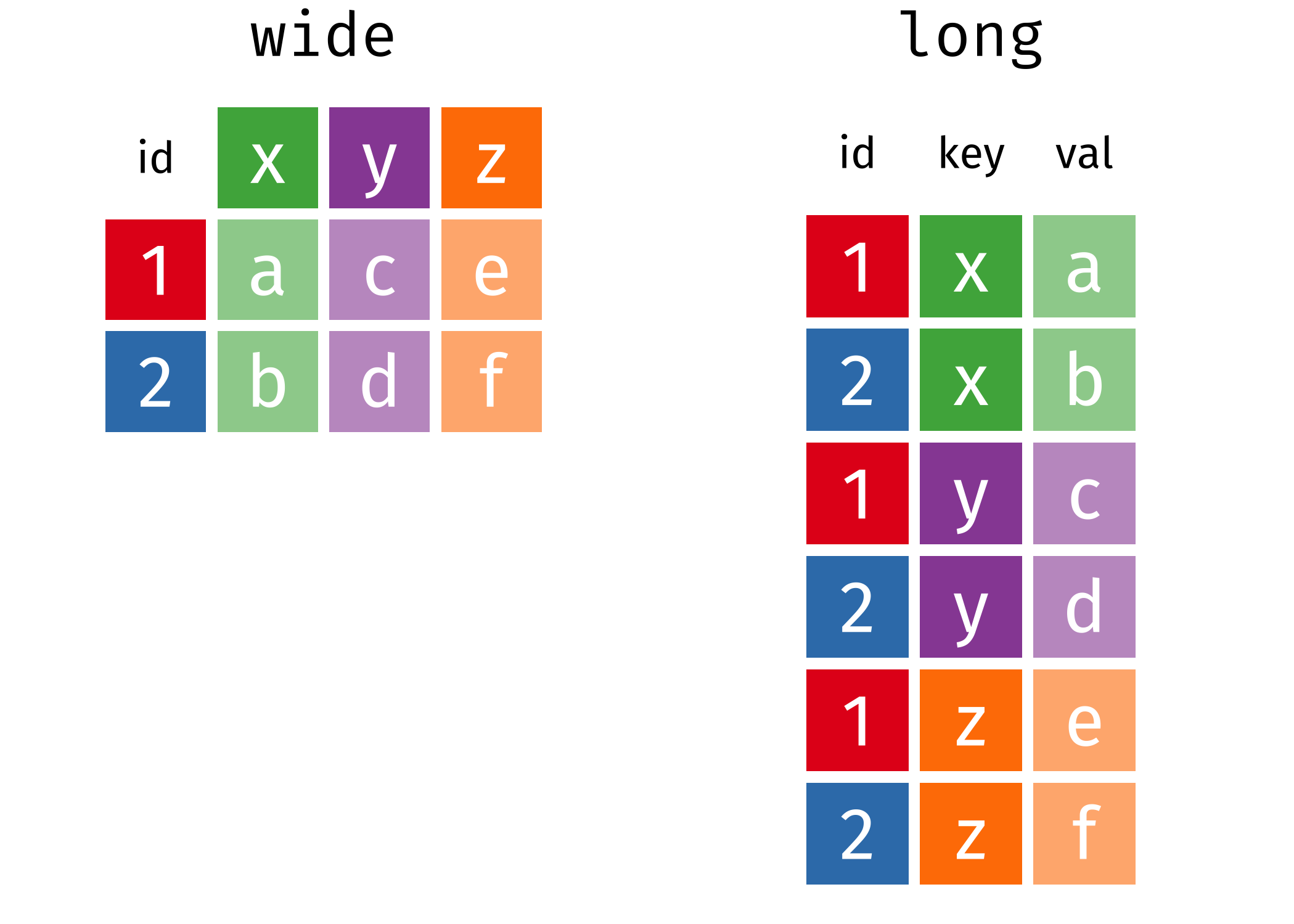
参数
cols,表示哪些列需要转换.参数
names_to,表示cols选取的这些列的名字,构成了新的一列,这里需要取一个名字.参数
values_to, 表示cols选取的这些列的值,构成了新的一列,这里也需要取一个名字.数据框总的信息量不会丢失
2 长表格变宽表格
spread()pivot_wider()
library(tidyverse)
plant_height <- data.frame(
  Day = 1:5,
  A = c(0.7, 1.0, 1.5, 1.8, 2.2),
  B = c(0.5, 0.7, 0.9, 1.3, 1.8),
  C = c(0.3, 0.6, 1.0, 1.2, 2.2),
  D = c(0.4, 0.7, 1.2, 1.5, 3.2)
)


plant_height
| Day | A | B | C | D |
|---|---|---|---|---|
| <int> | <dbl> | <dbl> | <dbl> | <dbl> |
| 1 | 0.7 | 0.5 | 0.3 | 0.4 |
| 2 | 1.0 | 0.7 | 0.6 | 0.7 |
| 3 | 1.5 | 0.9 | 1.0 | 1.2 |
| 4 | 1.8 | 1.3 | 1.2 | 1.5 |
| 5 | 2.2 | 1.8 | 2.2 | 3.2 |
melted <- plant_height %>%
  pivot_longer(cols = A:D,   # -Day or c(A, B, C, D) or c("A", "B", "C", "D")
               names_to = "plant",
               values_to = "height")
melted

melted1 <- gather(plant_height, variable, value, A:D)
melted1
| Day | plant | height |
|---|---|---|
| <int> | <chr> | <dbl> |
| 1 | A | 0.7 |
| 1 | B | 0.5 |
| 1 | C | 0.3 |
| 1 | D | 0.4 |
| 2 | A | 1.0 |
| 2 | B | 0.7 |
| 2 | C | 0.6 |
| 2 | D | 0.7 |
| 3 | A | 1.5 |
| 3 | B | 0.9 |
| 3 | C | 1.0 |
| 3 | D | 1.2 |
| 4 | A | 1.8 |
| 4 | B | 1.3 |
| 4 | C | 1.2 |
| 4 | D | 1.5 |
| 5 | A | 2.2 |
| 5 | B | 1.8 |
| 5 | C | 2.2 |
| 5 | D | 3.2 |
| Day | variable | value |
|---|---|---|
| <int> | <chr> | <dbl> |
| 1 | A | 0.7 |
| 2 | A | 1.0 |
| 3 | A | 1.5 |
| 4 | A | 1.8 |
| 5 | A | 2.2 |
| 1 | B | 0.5 |
| 2 | B | 0.7 |
| 3 | B | 0.9 |
| 4 | B | 1.3 |
| 5 | B | 1.8 |
| 1 | C | 0.3 |
| 2 | C | 0.6 |
| 3 | C | 1.0 |
| 4 | C | 1.2 |
| 5 | C | 2.2 |
| 1 | D | 0.4 |
| 2 | D | 0.7 |
| 3 | D | 1.2 |
| 4 | D | 1.5 |
| 5 | D | 3.2 |
melted %>%
  ggplot(aes(x=Day, y=height, color=plant))+
  geom_line()
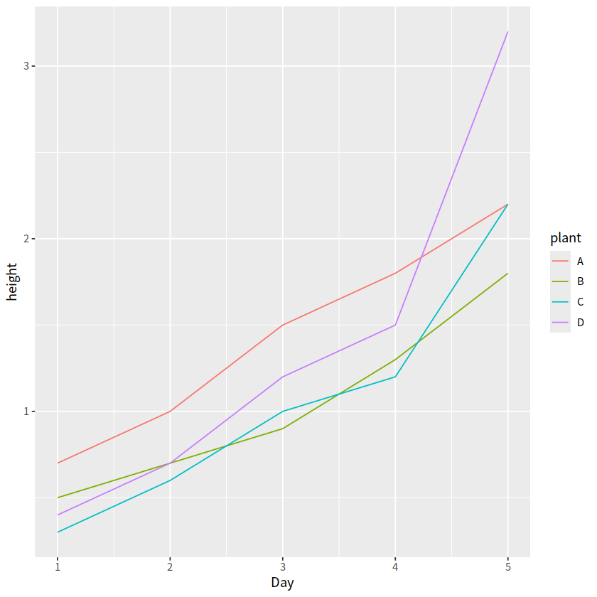
wide <- melted %>%
  pivot_wider(
  names_from = "plant",
  values_from = "height"
)
wide
| Day | A | B | C | D |
|---|---|---|---|---|
| <int> | <dbl> | <dbl> | <dbl> | <dbl> |
| 1 | 0.7 | 0.5 | 0.3 | 0.4 |
| 2 | 1.0 | 0.7 | 0.6 | 0.7 |
| 3 | 1.5 | 0.9 | 1.0 | 1.2 |
| 4 | 1.8 | 1.3 | 1.2 | 1.5 |
| 5 | 2.2 | 1.8 | 2.2 | 3.2 |
列名转换成多个变量
pivot_longer()中的names_pattern =指定表头属性pivot_wider()中的names_glue =指定转变后表头样式
plant_record <- data.frame(
         day = c(1L, 2L, 3L, 4L, 5L),
    A_height = c(1.1, 1.2, 1.3, 1.4, 1.5),
     A_width = c(2.1, 2.2, 2.3, 2.4, 2.5),
     A_depth = c(3.1, 3.2, 3.3, 3.4, 3.5),
    B_height = c(4.1, 4.2, 4.3, 4.4, 4.5),
     B_width = c(5.1, 5.2, 5.3, 5.4, 5.5),
     B_depth = c(6.1, 6.2, 6.3, 6.4, 6.5),
    C_height = c(7.1, 7.2, 7.3, 7.4, 7.5),
     C_width = c(8.1, 8.2, 8.3, 8.4, 8.5),
     C_depth = c(9.1, 9.2, 9.3, 9.4, 9.5)
)
plant_record
| day | A_height | A_width | A_depth | B_height | B_width | B_depth | C_height | C_width | C_depth |
|---|---|---|---|---|---|---|---|---|---|
| <int> | <dbl> | <dbl> | <dbl> | <dbl> | <dbl> | <dbl> | <dbl> | <dbl> | <dbl> |
| 1 | 1.1 | 2.1 | 3.1 | 4.1 | 5.1 | 6.1 | 7.1 | 8.1 | 9.1 |
| 2 | 1.2 | 2.2 | 3.2 | 4.2 | 5.2 | 6.2 | 7.2 | 8.2 | 9.2 |
| 3 | 1.3 | 2.3 | 3.3 | 4.3 | 5.3 | 6.3 | 7.3 | 8.3 | 9.3 |
| 4 | 1.4 | 2.4 | 3.4 | 4.4 | 5.4 | 6.4 | 7.4 | 8.4 | 9.4 |
| 5 | 1.5 | 2.5 | 3.5 | 4.5 | 5.5 | 6.5 | 7.5 | 8.5 | 9.5 |
我们想原始数据框的列名,转换成多个变量,比如A,B,C成为物种(species)变量,(height, width, depth)成为parameter变量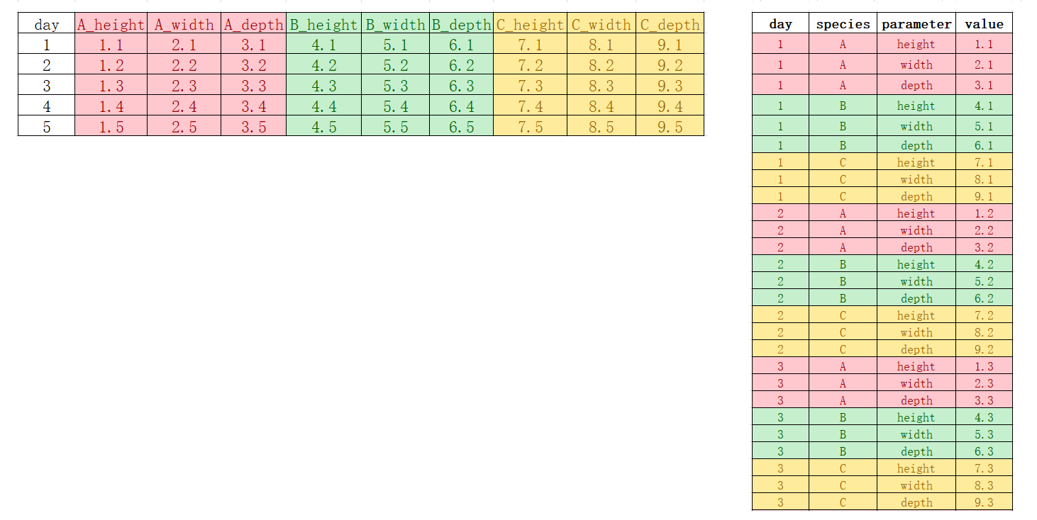
我们希望原始数据框的列名中,一部分进入变量,一部分保持原来的列名,比如,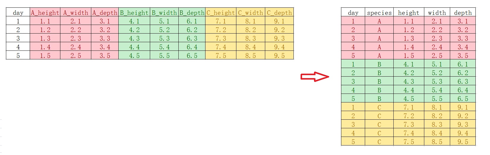
## pivot_longer()函数的实现列名转换成多个变量
plant_record %>%
  tidyr::pivot_longer(cols = !day,
                      names_to = c("species", "parameter"),
                      names_pattern = "(.*)_(.*)",
                      values_to = "value")

## pivot_longer()函数实现部分列名转变成变量,部分保持原来的列名
plant_record_longer <- plant_record %>%
  tidyr::pivot_longer(cols = !day,
                      names_to = c("species",".value"),
                      names_pattern = "(.*)_(.*)")
plant_record_longer
# 注意 .value 而不是value,说明这里不是单个列名,
# 而是匹配得到的多个值做列名
| day | species | parameter | value |
|---|---|---|---|
| <int> | <chr> | <chr> | <dbl> |
| 1 | A | height | 1.1 |
| 1 | A | width | 2.1 |
| 1 | A | depth | 3.1 |
| 1 | B | height | 4.1 |
| 1 | B | width | 5.1 |
| 1 | B | depth | 6.1 |
| 1 | C | height | 7.1 |
| 1 | C | width | 8.1 |
| 1 | C | depth | 9.1 |
| 2 | A | height | 1.2 |
| 2 | A | width | 2.2 |
| 2 | A | depth | 3.2 |
| 2 | B | height | 4.2 |
| 2 | B | width | 5.2 |
| 2 | B | depth | 6.2 |
| 2 | C | height | 7.2 |
| 2 | C | width | 8.2 |
| 2 | C | depth | 9.2 |
| 3 | A | height | 1.3 |
| 3 | A | width | 2.3 |
| 3 | A | depth | 3.3 |
| 3 | B | height | 4.3 |
| 3 | B | width | 5.3 |
| 3 | B | depth | 6.3 |
| 3 | C | height | 7.3 |
| 3 | C | width | 8.3 |
| 3 | C | depth | 9.3 |
| 4 | A | height | 1.4 |
| 4 | A | width | 2.4 |
| 4 | A | depth | 3.4 |
| 4 | B | height | 4.4 |
| 4 | B | width | 5.4 |
| 4 | B | depth | 6.4 |
| 4 | C | height | 7.4 |
| 4 | C | width | 8.4 |
| 4 | C | depth | 9.4 |
| 5 | A | height | 1.5 |
| 5 | A | width | 2.5 |
| 5 | A | depth | 3.5 |
| 5 | B | height | 4.5 |
| 5 | B | width | 5.5 |
| 5 | B | depth | 6.5 |
| 5 | C | height | 7.5 |
| 5 | C | width | 8.5 |
| 5 | C | depth | 9.5 |
| day | species | height | width | depth |
|---|---|---|---|---|
| <int> | <chr> | <dbl> | <dbl> | <dbl> |
| 1 | A | 1.1 | 2.1 | 3.1 |
| 1 | B | 4.1 | 5.1 | 6.1 |
| 1 | C | 7.1 | 8.1 | 9.1 |
| 2 | A | 1.2 | 2.2 | 3.2 |
| 2 | B | 4.2 | 5.2 | 6.2 |
| 2 | C | 7.2 | 8.2 | 9.2 |
| 3 | A | 1.3 | 2.3 | 3.3 |
| 3 | B | 4.3 | 5.3 | 6.3 |
| 3 | C | 7.3 | 8.3 | 9.3 |
| 4 | A | 1.4 | 2.4 | 3.4 |
| 4 | B | 4.4 | 5.4 | 6.4 |
| 4 | C | 7.4 | 8.4 | 9.4 |
| 5 | A | 1.5 | 2.5 | 3.5 |
| 5 | B | 4.5 | 5.5 | 6.5 |
| 5 | C | 7.5 | 8.5 | 9.5 |
变回去
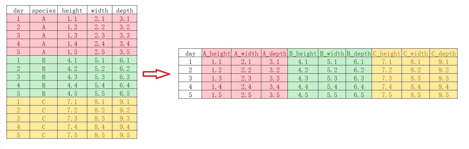
us_rent_income %>%
    pivot_wider(
      names_from = variable,
      names_glue = "{variable}_{.value}",
      values_from = c(estimate, moe))
| GEOID | NAME | income_estimate | rent_estimate | income_moe | rent_moe |
|---|---|---|---|---|---|
| <chr> | <chr> | <dbl> | <dbl> | <dbl> | <dbl> |
| 01 | Alabama | 24476 | 747 | 136 | 3 |
| 02 | Alaska | 32940 | 1200 | 508 | 13 |
| 04 | Arizona | 27517 | 972 | 148 | 4 |
| 05 | Arkansas | 23789 | 709 | 165 | 5 |
| 06 | California | 29454 | 1358 | 109 | 3 |
| 08 | Colorado | 32401 | 1125 | 109 | 5 |
| 09 | Connecticut | 35326 | 1123 | 195 | 5 |
| 10 | Delaware | 31560 | 1076 | 247 | 10 |
| 11 | District of Columbia | 43198 | 1424 | 681 | 17 |
| 12 | Florida | 25952 | 1077 | 70 | 3 |
| 13 | Georgia | 27024 | 927 | 106 | 3 |
| 15 | Hawaii | 32453 | 1507 | 218 | 18 |
| 16 | Idaho | 25298 | 792 | 208 | 7 |
| 17 | Illinois | 30684 | 952 | 83 | 3 |
| 18 | Indiana | 27247 | 782 | 117 | 3 |
| 19 | Iowa | 30002 | 740 | 143 | 4 |
| 20 | Kansas | 29126 | 801 | 208 | 5 |
| 21 | Kentucky | 24702 | 713 | 159 | 4 |
| 22 | Louisiana | 25086 | 825 | 155 | 4 |
| 23 | Maine | 26841 | 808 | 187 | 7 |
| 24 | Maryland | 37147 | 1311 | 152 | 5 |
| 25 | Massachusetts | 34498 | 1173 | 199 | 5 |
| 26 | Michigan | 26987 | 824 | 82 | 3 |
| 27 | Minnesota | 32734 | 906 | 189 | 4 |
| 28 | Mississippi | 22766 | 740 | 194 | 5 |
| 29 | Missouri | 26999 | 784 | 113 | 4 |
| 30 | Montana | 26249 | 751 | 206 | 9 |
| 31 | Nebraska | 30020 | 773 | 146 | 4 |
| 32 | Nevada | 29019 | 1017 | 213 | 6 |
| 33 | New Hampshire | 33172 | 1052 | 387 | 9 |
| 34 | New Jersey | 35075 | 1249 | 148 | 4 |
| 35 | New Mexico | 24457 | 809 | 214 | 6 |
| 36 | New York | 31057 | 1194 | 69 | 3 |
| 37 | North Carolina | 26482 | 844 | 111 | 3 |
| 38 | North Dakota | 32336 | 775 | 245 | 9 |
| 39 | Ohio | 27435 | 764 | 94 | 2 |
| 40 | Oklahoma | 26207 | 766 | 101 | 3 |
| 41 | Oregon | 27389 | 988 | 146 | 4 |
| 42 | Pennsylvania | 28923 | 885 | 119 | 3 |
| 44 | Rhode Island | 30210 | 957 | 259 | 6 |
| 45 | South Carolina | 25454 | 836 | 123 | 4 |
| 46 | South Dakota | 28821 | 696 | 276 | 7 |
| 47 | Tennessee | 25453 | 808 | 102 | 4 |
| 48 | Texas | 28063 | 952 | 110 | 2 |
| 49 | Utah | 27928 | 948 | 239 | 6 |
| 50 | Vermont | 29351 | 945 | 361 | 11 |
| 51 | Virginia | 32545 | 1166 | 202 | 5 |
| 53 | Washington | 32318 | 1120 | 113 | 4 |
| 54 | West Virginia | 23707 | 681 | 203 | 6 |
| 55 | Wisconsin | 29868 | 813 | 135 | 3 |
| 56 | Wyoming | 30854 | 828 | 342 | 11 |
| 72 | Puerto Rico | NA | 464 | NA | 6 |
注意
.value而不是value,说明这里不是单个列名,而是匹配得到的多个值做列名
plant_record_longer %>%
  pivot_wider(names_from = species,
              values_from = c(height, width, depth),
              names_glue = "{species}_{.value}")
| day | A_height | B_height | C_height | A_width | B_width | C_width | A_depth | B_depth | C_depth |
|---|---|---|---|---|---|---|---|---|---|
| <int> | <dbl> | <dbl> | <dbl> | <dbl> | <dbl> | <dbl> | <dbl> | <dbl> | <dbl> |
| 1 | 1.1 | 4.1 | 7.1 | 2.1 | 5.1 | 8.1 | 3.1 | 6.1 | 9.1 |
| 2 | 1.2 | 4.2 | 7.2 | 2.2 | 5.2 | 8.2 | 3.2 | 6.2 | 9.2 |
| 3 | 1.3 | 4.3 | 7.3 | 2.3 | 5.3 | 8.3 | 3.3 | 6.3 | 9.3 |
| 4 | 1.4 | 4.4 | 7.4 | 2.4 | 5.4 | 8.4 | 3.4 | 6.4 | 9.4 |
| 5 | 1.5 | 4.5 | 7.5 | 2.5 | 5.5 | 8.5 | 3.5 | 6.5 | 9.5 |
tidy data原则#
Hadley Wickhamt提出了数据科学tidy原则
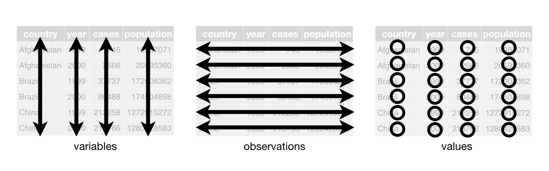
一切都是数据框,任何数据都可以规整
数据框的一列代表一个变量,数据框的一行代表一次观察
函数处理数据时,数据框进数据框出(函数的第一个参数始终为数据框)
根据Hadley Wickham的思想,这里的宽表格(plant_heigt和 wide)不是tidy的,只有长表格(long)才是tidy的,
melted
| Day | plant | height |
|---|---|---|
| <int> | <chr> | <dbl> |
| 1 | A | 0.7 |
| 1 | B | 0.5 |
| 1 | C | 0.3 |
| 1 | D | 0.4 |
| 2 | A | 1.0 |
| 2 | B | 0.7 |
| 2 | C | 0.6 |
| 2 | D | 0.7 |
| 3 | A | 1.5 |
| 3 | B | 0.9 |
| 3 | C | 1.0 |
| 3 | D | 1.2 |
| 4 | A | 1.8 |
| 4 | B | 1.3 |
| 4 | C | 1.2 |
| 4 | D | 1.5 |
| 5 | A | 2.2 |
| 5 | B | 1.8 |
| 5 | C | 2.2 |
| 5 | D | 3.2 |
fill()缺失值填充#
根据最近进行补齐
可以控制填充的方向
.direction = "up"
sales <- tibble::tribble(
  ~quarter, ~year, ~sales,
      "Q1",  2000,  66013,
      "Q2",    NA,  69182,
      "Q3",    NA,  53175,
      "Q4",    NA,  21001,
      "Q1",  2001,  46036,
      "Q2",    NA,  58842,
      "Q3",    NA,  44568,
      "Q4",    NA,  50197,
      "Q1",  2002,  39113,
      "Q2",    NA,  41668,
      "Q3",    NA,  30144,
      "Q4",    NA,  52897
  )
sales
| quarter | year | sales |
|---|---|---|
| <chr> | <dbl> | <dbl> |
| Q1 | 2000 | 66013 |
| Q2 | NA | 69182 |
| Q3 | NA | 53175 |
| Q4 | NA | 21001 |
| Q1 | 2001 | 46036 |
| Q2 | NA | 58842 |
| Q3 | NA | 44568 |
| Q4 | NA | 50197 |
| Q1 | 2002 | 39113 |
| Q2 | NA | 41668 |
| Q3 | NA | 30144 |
| Q4 | NA | 52897 |
sales %>% fill(year)
sales %>% fill(year, .direction="up")
| quarter | year | sales |
|---|---|---|
| <chr> | <dbl> | <dbl> |
| Q1 | 2000 | 66013 |
| Q2 | 2000 | 69182 |
| Q3 | 2000 | 53175 |
| Q4 | 2000 | 21001 |
| Q1 | 2001 | 46036 |
| Q2 | 2001 | 58842 |
| Q3 | 2001 | 44568 |
| Q4 | 2001 | 50197 |
| Q1 | 2002 | 39113 |
| Q2 | 2002 | 41668 |
| Q3 | 2002 | 30144 |
| Q4 | 2002 | 52897 |
| quarter | year | sales |
|---|---|---|
| <chr> | <dbl> | <dbl> |
| Q1 | 2000 | 66013 |
| Q2 | 2001 | 69182 |
| Q3 | 2001 | 53175 |
| Q4 | 2001 | 21001 |
| Q1 | 2001 | 46036 |
| Q2 | 2002 | 58842 |
| Q3 | 2002 | 44568 |
| Q4 | 2002 | 50197 |
| Q1 | 2002 | 39113 |
| Q2 | NA | 41668 |
| Q3 | NA | 30144 |
| Q4 | NA | 52897 |
expand() 与 complete()#
expand()指定数据框的若干列,根据其向量元素值,产生所有可能的交叉组合nesting()用于限定只产生数据框已出现的组合
complete()补全,可以看作是expand(nesting()) + fill()数据在
complete补全的时候,会面临有两种缺失值:1 补位的时候造成的空缺
2 数据原先就存在缺失值
3 补位的时候造成的空缺,可通过
fill = list(x = 0)控制填充4 数据原先就存在缺失值,最好通过
explicit = FALSE显式地控制是否填充
df <- tibble::tribble(
  ~x, ~y, ~z,
  1L, 1L, 4L,
  1L, 2L, 5L,
  2L, 1L, NA,
  3L, 2L, 6L
)
df
df %>% expand(x,y)
df %>% expand(nesting(x,y))
df %>% expand(nesting(x,y), z)
| x | y | z |
|---|---|---|
| <int> | <int> | <int> |
| 1 | 1 | 4 |
| 1 | 2 | 5 |
| 2 | 1 | NA |
| 3 | 2 | 6 |
| x | y |
|---|---|
| <int> | <int> |
| 1 | 1 |
| 1 | 2 |
| 2 | 1 |
| 2 | 2 |
| 3 | 1 |
| 3 | 2 |
| x | y |
|---|---|
| <int> | <int> |
| 1 | 1 |
| 1 | 2 |
| 2 | 1 |
| 3 | 2 |
| x | y | z |
|---|---|---|
| <int> | <int> | <int> |
| 1 | 1 | 4 |
| 1 | 1 | 5 |
| 1 | 1 | 6 |
| 1 | 1 | NA |
| 1 | 2 | 4 |
| 1 | 2 | 5 |
| 1 | 2 | 6 |
| 1 | 2 | NA |
| 2 | 1 | 4 |
| 2 | 1 | 5 |
| 2 | 1 | 6 |
| 2 | 1 | NA |
| 3 | 2 | 4 |
| 3 | 2 | 5 |
| 3 | 2 | 6 |
| 3 | 2 | NA |
df %>% complete(x, y)
df %>% complete(x, y, fill=list(z=0))
df %>% complete(x, y, fill = list(z = 0), explicit = FALSE)
| x | y | z |
|---|---|---|
| <int> | <int> | <int> |
| 1 | 1 | 4 |
| 1 | 2 | 5 |
| 2 | 1 | NA |
| 2 | 2 | NA |
| 3 | 1 | NA |
| 3 | 2 | 6 |
| x | y | z |
|---|---|---|
| <int> | <int> | <int> |
| 1 | 1 | 4 |
| 1 | 2 | 5 |
| 2 | 1 | 0 |
| 2 | 2 | 0 |
| 3 | 1 | 0 |
| 3 | 2 | 6 |
| x | y | z |
|---|---|---|
| <int> | <int> | <int> |
| 1 | 1 | 4 |
| 1 | 2 | 5 |
| 2 | 1 | NA |
| 2 | 2 | 0 |
| 3 | 1 | 0 |
| 3 | 2 | 6 |
expand_grid() 与 crossing()#
expand_grid()产生一个新的数据框,每行对应着向量元素的所有交叉组合向量换成数据框也可以,其结果就是数据框行与元素的交叉组合
crossing()可以看作是expand_grid() + distinct(), 即crossing()在完成交叉组合之后会自动去重
expand_grid(x=c(1,1,2), y= 1:2)
crossing(x=c(1,1,2), y=1:2)
| x | y |
|---|---|
| <dbl> | <int> |
| 1 | 1 |
| 1 | 2 |
| 1 | 1 |
| 1 | 2 |
| 2 | 1 |
| 2 | 2 |
| x | y |
|---|---|
| <dbl> | <int> |
| 1 | 1 |
| 1 | 2 |
| 2 | 1 |
| 2 | 2 |
separate()与unite()#
以提供的分隔符分隔或合并某些列
有时候分隔符搞不定的,可以用正则表达式,将捕获的每组弄成一列
tb <- tibble::tribble(
  ~day, ~price,
  1,   "30-45",
  2,   "40-95",
  3,   "89-65",
  4,   "45-63",
  5,   "52-42"
)
tb %>%
  separate(price, into=c("low", "high"), sep="-") %>%
  unite(col="price", c(low, high), sep=":", remove=FALSE)
| day | price | low | high |
|---|---|---|---|
| <dbl> | <chr> | <chr> | <chr> |
| 1 | 30:45 | 30 | 45 |
| 2 | 40:95 | 40 | 95 |
| 3 | 89:65 | 89 | 65 |
| 4 | 45:63 | 45 | 63 |
| 5 | 52:42 | 52 | 42 |
## 有时候分隔符搞不定的,可以用正则表达式,将捕获的每组弄成一列
dfc <- tibble(x = c("1-12week", "1-10wk", "5-12w", "01-05weeks"))
dfc

dfc %>% tidyr::extract(
  x,
  c("start", "end", "letter"), "(\\d+)-(\\d+)([a-z]+)",
  remove = FALSE
)
| x |
|---|
| <chr> |
| 1-12week |
| 1-10wk |
| 5-12w |
| 01-05weeks |
| x | start | end | letter |
|---|---|---|---|
| <chr> | <chr> | <chr> | <chr> |
| 1-12week | 1 | 12 | week |
| 1-10wk | 1 | 10 | wk |
| 5-12w | 5 | 12 | w |
| 01-05weeks | 01 | 05 | weeks |
删除缺失值所在行drop_na()与replace_na()#
drop_na()删除有缺失值的所有row,等效于filter(across(everything(), ~!is.na(.x))),可单独使用df %>% drop_na()删除df中的缺失值也可指定某列,只删除该列存在缺失值的行
replace_na()coalesce()替换缺失值x = replace_na(x, 0)将x列的缺失值替换为0, 可在mutate()等函数中使用
df <- tibble::tribble(
    ~name,     ~type, ~score, ~extra,
  "Alice", "english",     80,     10,
  "Alice",    "math",     NA,      5,
    "Bob", "english",     NA,      9,
    "Bob",    "math",     69,     NA,
  "Carol", "english",     80,     10,
  "Carol",    "math",     90,      5
  )

# 如果score列中有缺失值NA,就删除所在的row
df %>%
  filter(!is.na(score))

df %>%
  filter(
    across(score, ~ !is.na(.x))
  )
| name | type | score | extra |
|---|---|---|---|
| <chr> | <chr> | <dbl> | <dbl> |
| Alice | english | 80 | 10 |
| Bob | math | 69 | NA |
| Carol | english | 80 | 10 |
| Carol | math | 90 | 5 |
Warning message:
“Using `across()` in `filter()` was deprecated in dplyr 1.0.8.
ℹ Please use `if_any()` or `if_all()` instead.”
| name | type | score | extra |
|---|---|---|---|
| <chr> | <chr> | <dbl> | <dbl> |
| Alice | english | 80 | 10 |
| Bob | math | 69 | NA |
| Carol | english | 80 | 10 |
| Carol | math | 90 | 5 |
# 所有列,如果有缺失值NA,就删除所在的row
df %>%
  filter(
    across(everything(), ~!is.na(.x))
  )

# 更简便的方法
df %>%
  drop_na()
# 也可指定某咧
df %>%
  drop_na(score)
Warning message:
“Using `across()` in `filter()` was deprecated in dplyr 1.0.8.
ℹ Please use `if_any()` or `if_all()` instead.”
| name | type | score | extra |
|---|---|---|---|
| <chr> | <chr> | <dbl> | <dbl> |
| Alice | english | 80 | 10 |
| Carol | english | 80 | 10 |
| Carol | math | 90 | 5 |
| name | type | score | extra |
|---|---|---|---|
| <chr> | <chr> | <dbl> | <dbl> |
| Alice | english | 80 | 10 |
| Carol | english | 80 | 10 |
| Carol | math | 90 | 5 |
| name | type | score | extra |
|---|---|---|---|
| <chr> | <chr> | <dbl> | <dbl> |
| Alice | english | 80 | 10 |
| Bob | math | 69 | NA |
| Carol | english | 80 | 10 |
| Carol | math | 90 | 5 |
# 将score替换为0分
df
df %>%
  mutate(score = replace_na(score, 0))
df %>%
  mutate(score = coalesce(score, 0))
| name | type | score | extra |
|---|---|---|---|
| <chr> | <chr> | <dbl> | <dbl> |
| Alice | english | 80 | 10 |
| Alice | math | NA | 5 |
| Bob | english | NA | 9 |
| Bob | math | 69 | NA |
| Carol | english | 80 | 10 |
| Carol | math | 90 | 5 |
| name | type | score | extra |
|---|---|---|---|
| <chr> | <chr> | <dbl> | <dbl> |
| Alice | english | 80 | 10 |
| Alice | math | 0 | 5 |
| Bob | english | 0 | 9 |
| Bob | math | 69 | NA |
| Carol | english | 80 | 10 |
| Carol | math | 90 | 5 |
| name | type | score | extra |
|---|---|---|---|
| <chr> | <chr> | <dbl> | <dbl> |
| Alice | english | 80 | 10 |
| Alice | math | 0 | 5 |
| Bob | english | 0 | 9 |
| Bob | math | 69 | NA |
| Carol | english | 80 | 10 |
| Carol | math | 90 | 5 |
df %>%
  mutate(
    across(c(score, extra), ~ replace_na(.x,0))
  )
df %>%
  mutate(
    across(c(score, extra), ~ coalesce(.x,0)))
| name | type | score | extra |
|---|---|---|---|
| <chr> | <chr> | <dbl> | <dbl> |
| Alice | english | 80 | 10 |
| Alice | math | 0 | 5 |
| Bob | english | 0 | 9 |
| Bob | math | 69 | 0 |
| Carol | english | 80 | 10 |
| Carol | math | 90 | 5 |
| name | type | score | extra |
|---|---|---|---|
| <chr> | <chr> | <dbl> | <dbl> |
| Alice | english | 80 | 10 |
| Alice | math | 0 | 5 |
| Bob | english | 0 | 9 |
| Bob | math | 69 | 0 |
| Carol | english | 80 | 10 |
| Carol | math | 90 | 5 |
df %>%
  mutate(
    score = replace_na(score, mean(score, na.rm=TRUE))
  )

## 也可用if_else()来做
df %>%
  mutate(
    score = if_else(is.na(score), mean(score, na.rm=TRUE), score)
  )
| name | type | score | extra |
|---|---|---|---|
| <chr> | <chr> | <dbl> | <dbl> |
| Alice | english | 80.00 | 10 |
| Alice | math | 79.75 | 5 |
| Bob | english | 79.75 | 9 |
| Bob | math | 69.00 | NA |
| Carol | english | 80.00 | 10 |
| Carol | math | 90.00 | 5 |
| name | type | score | extra |
|---|---|---|---|
| <chr> | <chr> | <dbl> | <dbl> |
| Alice | english | 80.00 | 10 |
| Alice | math | 79.75 | 5 |
| Bob | english | 79.75 | 9 |
| Bob | math | 69.00 | NA |
| Carol | english | 80.00 | 10 |
| Carol | math | 90.00 | 5 |