因子型变量_数据框_函数式编程purrr包#
什么是因子#
因子是把数据进行分类并标记为不同层级(level,有时候也翻译成因子水平, 我个人觉得翻译为层级,更接近它的特性,因此,我都会用层级来描述)的数据对象,他们可以存储字符串和整数。因子类型有三个属性:
存储类别的数据类型
离散变量
因子的层级是有限的,只能取因子层级中的值或缺失(
NA)
创建因子#
因子层级会自动按照字符串的字母顺序排序,比如
high low medium。也可以用levels=c()指定顺序不属于因子层级中的值, 会被当作缺省值
NA
library(tidyverse)
── Attaching core tidyverse packages ───────────────────────────────────────────────────────────────────────────────────────────────────────────────────────── tidyverse 2.0.0 ──
✔ dplyr     1.1.4     ✔ readr     2.1.5
✔ forcats   1.0.0     ✔ stringr   1.5.1
✔ ggplot2   3.5.0     ✔ tibble    3.2.1
✔ lubridate 1.9.3     ✔ tidyr     1.3.1
✔ purrr     1.0.2
── Conflicts ─────────────────────────────────────────────────────────────────────────────────────────────────────────────────────────────────────────── tidyverse_conflicts() ──
✖ dplyr::filter() masks stats::filter()
✖ dplyr::lag()    masks stats::lag()
ℹ Use the conflicted package (<http://conflicted.r-lib.org/>) to force all conflicts to become errors
library(palmerpenguins)
income <- c("low", "high", "medium", "medium", "low", "high",  "high")
factor(income)
- low
- high
- medium
- medium
- low
- high
- high
Levels:
- 'high'
- 'low'
- 'medium'
## 指定顺序
factor(income, levels=c("low", "high", "medium"))
- low
- high
- medium
- medium
- low
- high
- high
Levels:
- 'low'
- 'high'
- 'medium'
factor(income, levels=c("low", "high"))
- low
- high
- <NA>
- <NA>
- low
- high
- high
Levels:
- 'low'
- 'high'
相比较字符串而言,因子类型更容易处理,因此很多函数会自动的将字符串转换为因子来处理,但事实上,这也会造成,不想当做因子的却又当做了因子的情形
最典型的是在R 4.0之前,data.frame()中stringsAsFactors选项,默认将字符串类型转换为因子类型,但这个默认也带来一些不方便,因此在R 4.0之后取消了这个默认。
在tidyverse集合里,有专门处理因子的宏包forcats
library(forcats)
调整因子顺序#
因子层级默认是按照字母顺序排序
fct_relevel()指定因子顺序after=Inf将某个因子移到最后面
fct_inorder()按照字符串第一次出现的次序fct_reorder()按照其他变量的升序排序.fun=指定函数fct_rev()按照因子层级的逆序排序fct_infreq()按照因子频率排序,从大到小fct_rev(fct_infreq())按照因子频率排序,从小到大
income <- c("low", "high", "medium", "medium", "low", "high",  "high")
x <- factor(income)
x
# 指定顺序
x %>% fct_relevel(c("high", "medium", "low"))
x %>% fct_relevel("medium")
x %>% fct_relevel("medium", after=Inf)

# 按照字符串第一次出现的次序
x %>% fct_inorder()
- low
- high
- medium
- medium
- low
- high
- high
Levels:
- 'high'
- 'low'
- 'medium'
- low
- high
- medium
- medium
- low
- high
- high
Levels:
- 'high'
- 'medium'
- 'low'
- low
- high
- medium
- medium
- low
- high
- high
Levels:
- 'medium'
- 'high'
- 'low'
- low
- high
- medium
- medium
- low
- high
- high
Levels:
- 'high'
- 'low'
- 'medium'
- low
- high
- medium
- medium
- low
- high
- high
Levels:
- 'low'
- 'high'
- 'medium'
# 按照其他变量的中位数的升序排序
x %>% fct_reorder(c(1:7), .fun=median)
- low
- high
- medium
- medium
- low
- high
- high
Levels:
- 'low'
- 'medium'
- 'high'
应用#
调整因子层级有什么用呢?
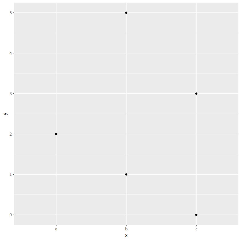
这个功能在ggplot可视化中调整分类变量的顺序非常方便
d <- tibble(
  x = c("a","a", "b", "b", "c", "c"),
  y = c(2, 2, 1, 5,  0, 3)

)
d
| x | y |
|---|---|
| <chr> | <dbl> |
| a | 2 |
| a | 2 |
| b | 1 |
| b | 5 |
| c | 0 |
| c | 3 |
d %>%
  ggplot(aes(x = x, y = y))+
  geom_point()
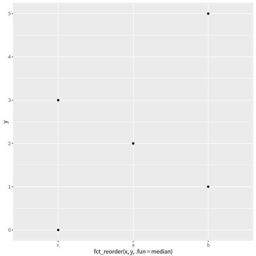
fct_reorder()#
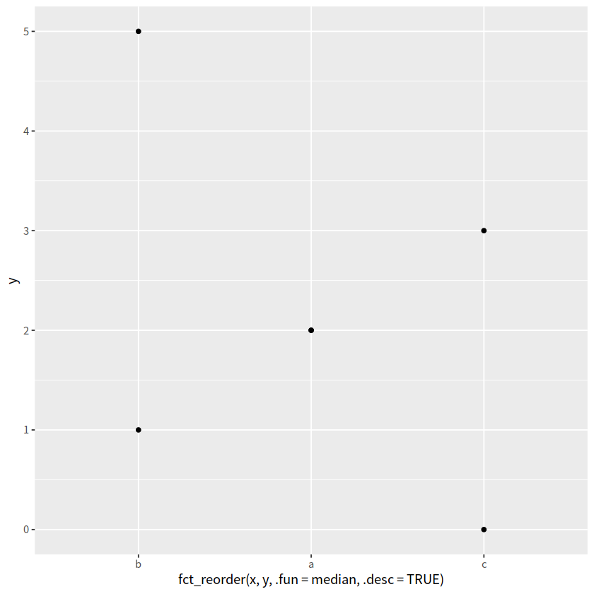
fct_reorder(x, y, .fun=median)可以让x的顺序按照x中每个分类变量对应y值的中位数升序排序.desc = TRUE颠倒顺序
d %>%
  ggplot(aes(x = fct_reorder(x, y, .fun=median), y = y)) +
  geom_point()
d %>%
ggplot(aes(x = fct_reorder(x,y, .fun=median, .desc=TRUE), y = y)) +
geom_point()
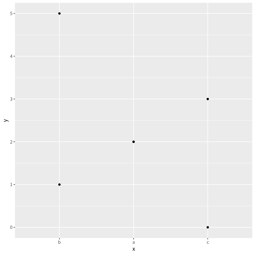
d %>%
mutate(x = fct_reorder(x, y, .fun=median, .desc=TRUE)) %>%
ggplot(aes(x = x, y = y)) +
geom_point()
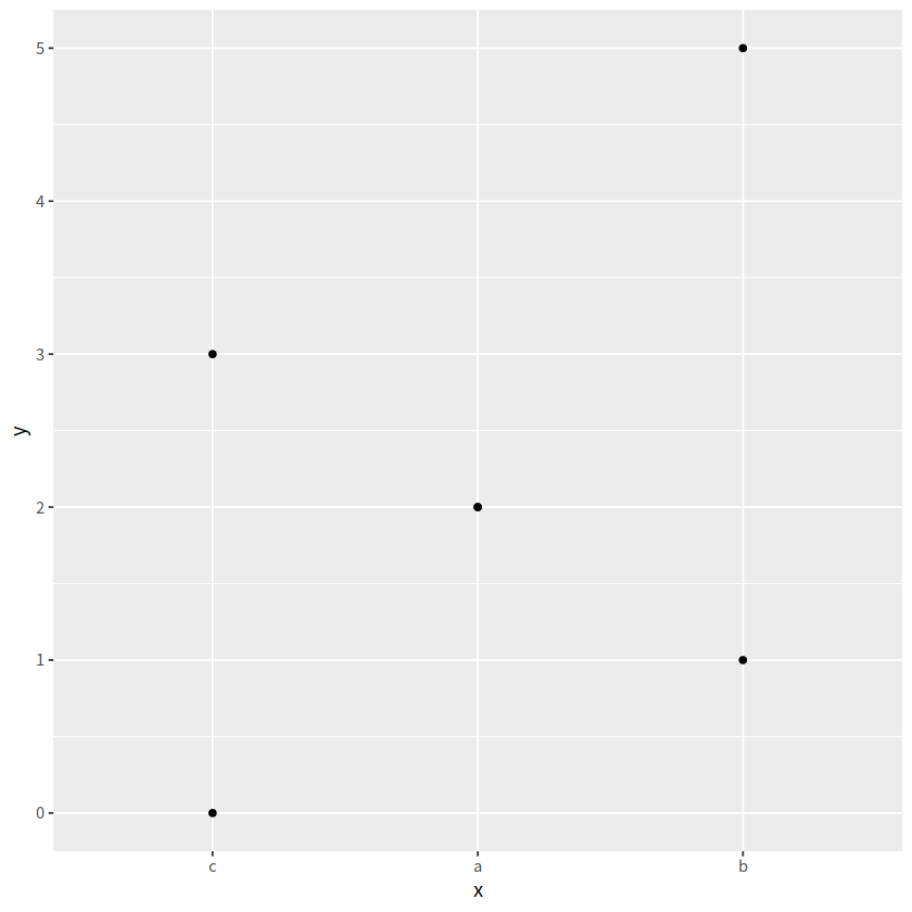
fct_rev()#
按照因子层级的逆序排序
d %>%
  mutate(x = fct_rev(x)) %>%
  ggplot(aes(x, y)) +
  geom_point()
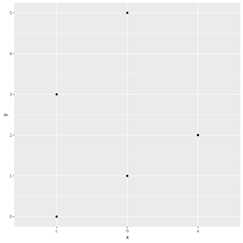
fct_relevel()#
d %>%
  mutate(
    x = fct_relevel(x, c("c", "a", "b"))
  ) %>%
  ggplot(aes(x, y))+
  geom_point()
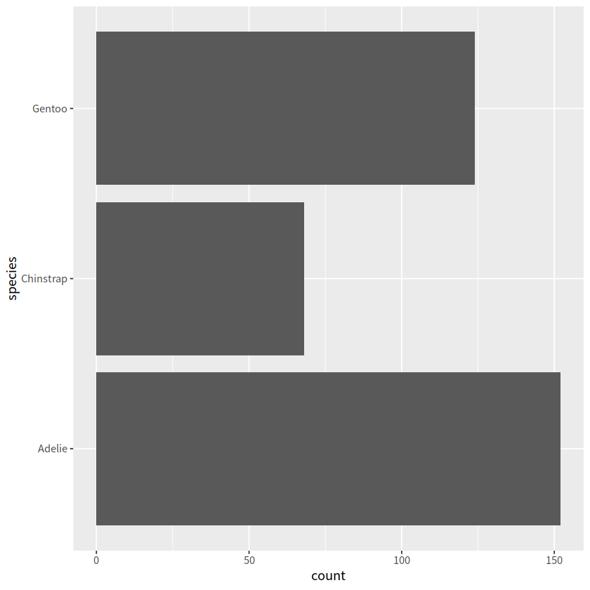
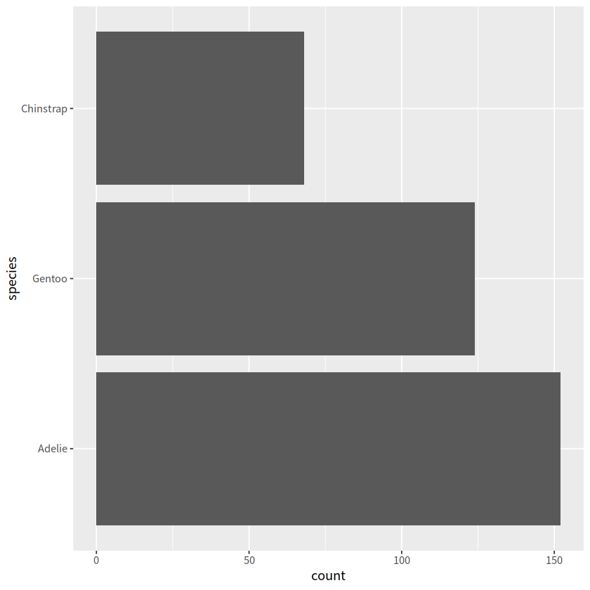
可视化中应用#
library(palmerpenguins)

ggplot(penguins, aes(y=species))+
  geom_bar()
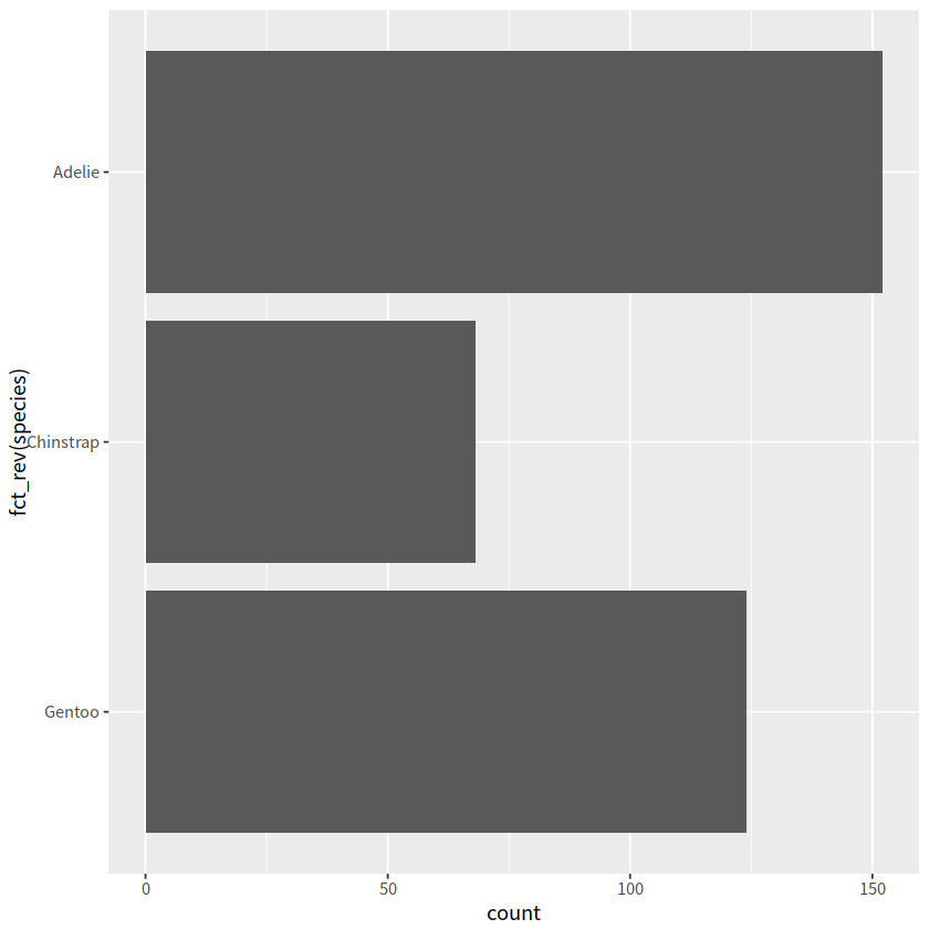
# 按species逆序
ggplot(penguins, aes(y = fct_rev(species)))+
  geom_bar()
penguins %>%
count(species) %>%
pull(species)
penguins %>%
count(species) %>%
mutate(species = fct_relevel(species, c("Chinstrap", "Gentoo", "Adelie"))) %>%
pull(species)
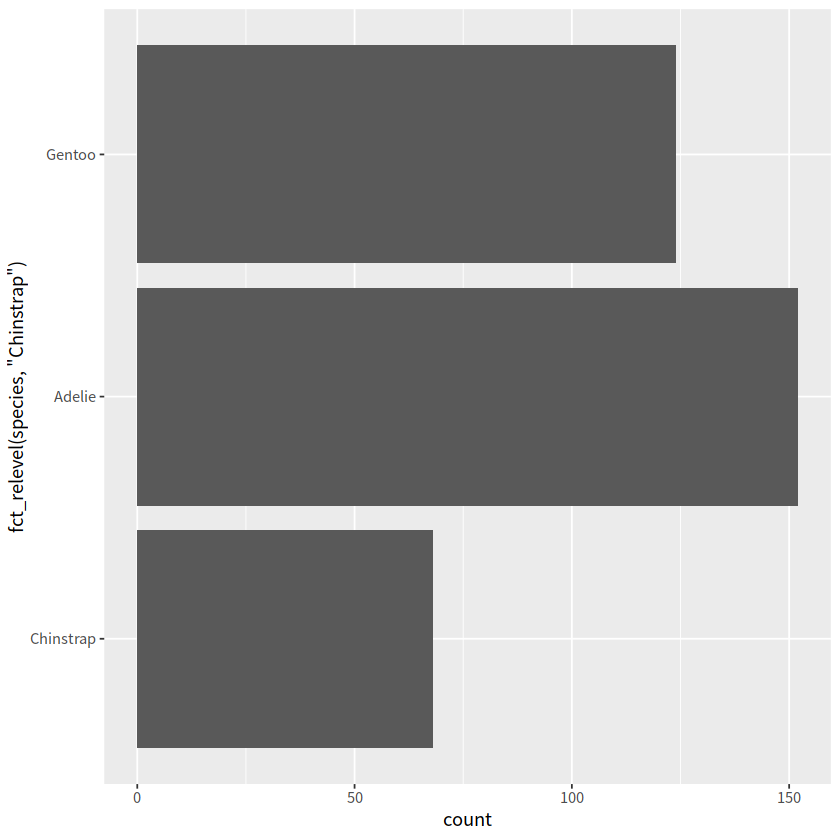
# 把Chinstrap移到前面, 其他顺序不变
ggplot(penguins, aes(y = fct_relevel(species, "Chinstrap"))) +
geom_bar()
- Adelie
- Chinstrap
- Gentoo
Levels:
- 'Adelie'
- 'Chinstrap'
- 'Gentoo'
- Adelie
- Chinstrap
- Gentoo
Levels:
- 'Chinstrap'
- 'Gentoo'
- 'Adelie'
# Use order "Chinstrap", "Gentoo", "Adelie"
ggplot(penguins, aes(y = fct_relevel(species, "Chinstrap", "Gentoo", "Adelie"))) +
  geom_bar()
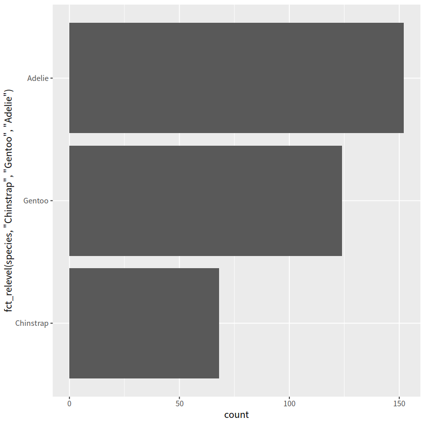
penguins %>%
  mutate(species = fct_relevel(species, "Chinstrap", "Gentoo", "Adelie")) %>%
  ggplot(aes( y = species))+
  geom_bar()

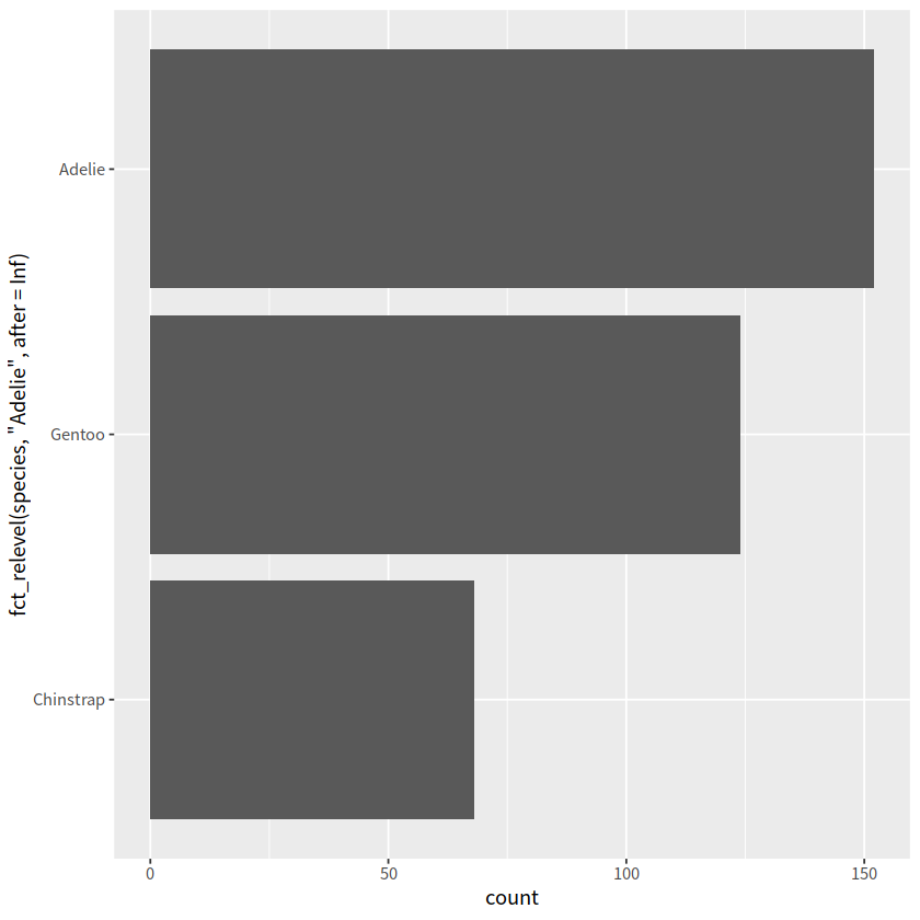
# 把Adelie放到最后
ggplot(penguins, aes(y = fct_relevel(species, "Adelie", after=Inf)))+
  geom_bar()
# fct_infreq() 按照因子频率,从小到大
penguins %>%
  mutate(species = fct_infreq(species)) %>%
  ggplot(aes(y = species))+
  geom_bar()

penguins %>%
  mutate(species = fct_rev(fct_infreq(species))) %>%
  ggplot(aes(y = species))+
  geom_bar()
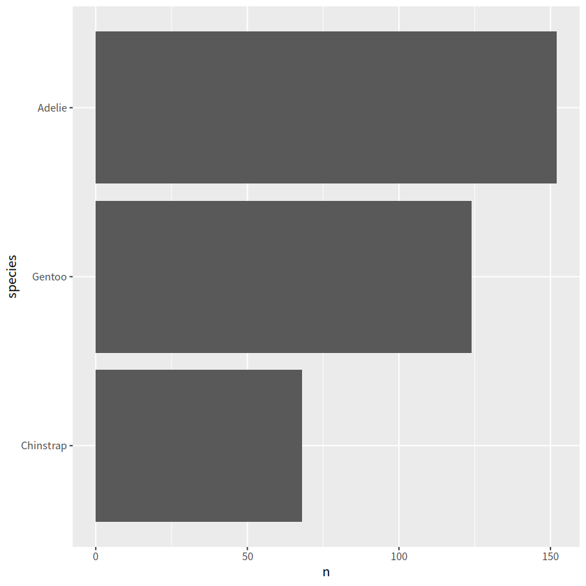
# n是count()函数产生的结果
penguins %>%
  count(species) %>%
  mutate(species = fct_reorder(species, n)) %>%
  ggplot(aes(n, species))+
  geom_col()
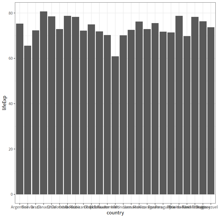
# 画出的2007年美洲人口寿命的柱状图,要求从高到低排序

library(gapminder) # install.packages("gapminder")
gapminder %>%
  filter(year == 2007 & continent == "Americas") %>%
  ggplot(aes(x = country, y = lifeExp))+
  geom_col()+
  theme_bw()
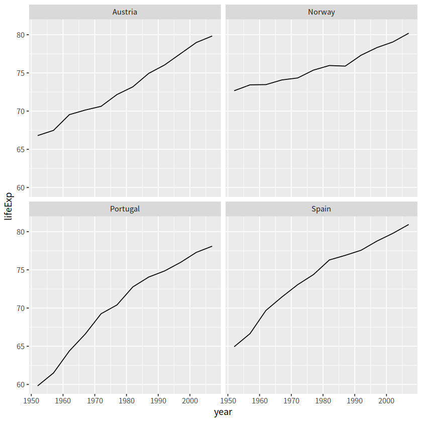
# 四个国家人口寿命的变化图
gapminder %>%
  filter(country %in% c("Norway", "Portugal", "Spain", "Austria")) %>%
  ggplot(aes(year, lifeExp)) +
  geom_line() +
  facet_wrap(vars(country), nrow = 2)
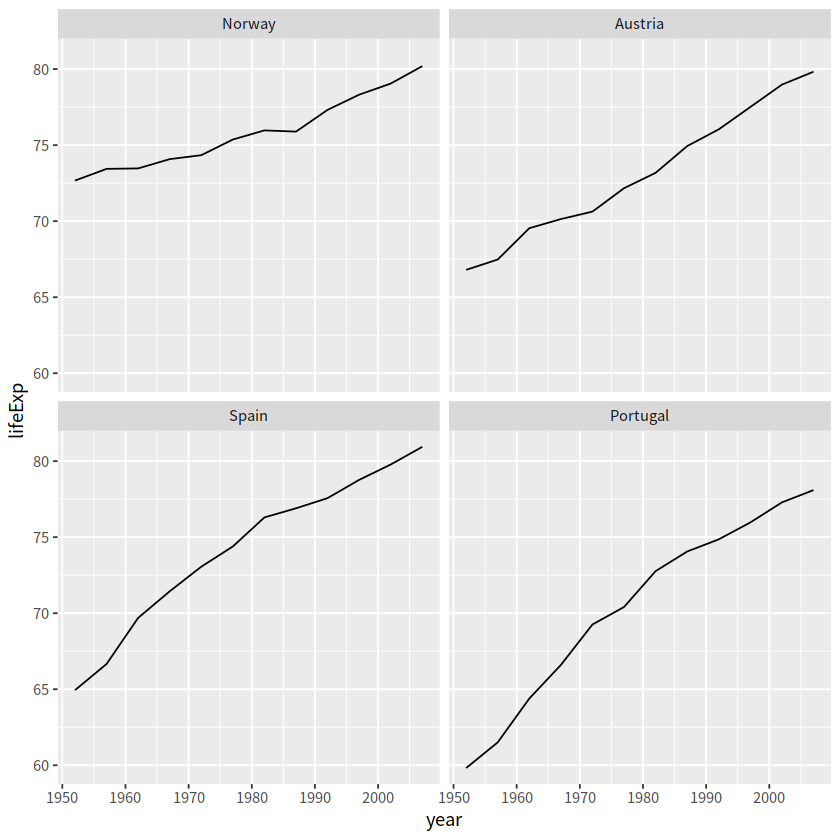
# 按每个国家寿命的中位数
gapminder %>%
  filter(country %in% c("Norway", "Portugal", "Spain", "Austria")) %>%
  mutate(country = fct_reorder(country, lifeExp, .fun=median)) %>%
  ggplot(aes(year, lifeExp)) +
  geom_line() +
  facet_wrap(vars(country), nrow = 2)

# 按每个国家寿命差(最大值减去最小值)
cha <- function(x){
    max(x) - min(x)
}

gapminder %>%
  filter(country %in% c("Norway", "Portugal", "Spain", "Austria")) %>%
  mutate(country = fct_reorder(country, lifeExp, .fun=cha)) %>%
  ggplot(aes(year, lifeExp)) +
  geom_line() +
  facet_wrap(vars(country), nrow = 2)
简单数据框#
tidyverse 家族#
前面陆续介绍了tidyverse家族,家庭主要成员包括
功能 |
宏包 |
|---|---|
有颜值担当 |
|
数据处理王者 |
|
数据转换专家 |
|
数据载入利器 |
|
循环加速器 |
|
强化数据框 |
|
字符串处理 |
|
因子处理 |
|
人性化的tibble#
tibble是用来替换data.frame类型的扩展的数据框tibble继承了data.frame,是弱类型的。换句话说,tibble是data.frame的子类型tibble与data.frame有相同的语法,使用起来更方便tibble更早的检查数据,方便写出更干净、更多富有表现力的代码
tibble对data.frame做了重新的设定:
tibble,不关心输入类型,可存储任意类型,包括list类型tibble,没有行名设置row.namestibble,支持任意的列名tibble,会自动添加列名tibble,类型只能回收长度为1的输入tibble,会懒加载参数,并按顺序运行tibble,是tbl_df类型
tibble 与 data.frame#
# 传统创建数据框
data.frame(
  a = 1:5,
  b = letters[1:5]
)
| a | b |
|---|---|
| <int> | <chr> |
| 1 | a |
| 2 | b |
| 3 | c |
| 4 | d |
| 5 | e |
发现,data.frame()会自动将字符串型的变量转换成因子型,如果想保持原来的字符串型,就得
data.frame(
  a = 1:5,
  b = letters[1:5],
  stringsAsFactors = FALSE
)
| a | b |
|---|---|
| <int> | <chr> |
| 1 | a |
| 2 | b |
| 3 | c |
| 4 | d |
| 5 | e |
Note: - 在R 4.0 后,data.frame() 不会将字符串型变量自动转换成因子型
用tibble创建数据框,不会这么麻烦,输出的就是原来的字符串类型
tibble(
  a = 1:5,
  b = letters[1:5]
)
| a | b |
|---|---|
| <int> | <chr> |
| 1 | a |
| 2 | b |
| 3 | c |
| 4 | d |
| 5 | e |
构建两个有关联的变量,传统的data.frame()会报错
tb <- tibble(
  x = 1:3,
  y = x+2)
tb

df <- data.frame(
  x = 1:3,
  y = x+2
)
| x | y |
|---|---|
| <int> | <dbl> |
| 1 | 3 |
| 2 | 4 |
| 3 | 5 |
Warning message in Ops.factor(x, 2):
“‘+’ not meaningful for factors”
Error in data.frame(x = 1:3, y = x + 2): 参数值意味着不同的行数: 3, 7
Traceback:

1. data.frame(x = 1:3, y = x + 2)
2. stop(gettextf("arguments imply differing number of rows: %s",
 .     paste(unique(nrows), collapse = ", ")), domain = NA)
tibble用缩写定义了7种类型:
类型 |
含义 |
|---|---|
|
代表 |
|
代表 |
|
代表 |
|
代表日期+时间( |
|
代表逻辑判断 |
|
代表因子类型 |
|
代表日期 |
tibble数据操作#
1 创建tibble#
tibble()创建方式和data.frame()一样tibble::tribble()更加直观
# tibble()创建一个tibble类型的data.frame:
tibble(a = 1:5, b = letters[1:5])
tibble(a = 1:5,
      b = 10:14,
      c = a + b)
| a | b |
|---|---|
| <int> | <chr> |
| 1 | a |
| 2 | b |
| 3 | c |
| 4 | d |
| 5 | e |
| a | b | c |
|---|---|---|
| <int> | <int> | <int> |
| 1 | 10 | 11 |
| 2 | 11 | 13 |
| 3 | 12 | 15 |
| 4 | 13 | 17 |
| 5 | 14 | 19 |
# 为了让每列更加直观,也可以tribble()创建,数据量不大的时候
tibble::tribble(
  ~x , ~y, ~z,
  "a", 2, 3.6,
  "b", 1, 8.5
)
| x | y | z |
|---|---|---|
| <chr> | <dbl> | <dbl> |
| a | 2 | 3.6 |
| b | 1 | 8.5 |
2 转换成tibble类型#
转换成tibble类型意思就是说,刚开始不是tibble, 现在转换成tibble, 包括
data.frame转换成tibbleas_tibble()runif(n, min=0, max=1)生成n个0-1之间的均匀分布随机数as.data.frame()转回去
vector转换成tibblelist转换成tibbleas.list()转回去
matrix转换成tibbletibble转回matrix?as.matrix()
# data.frame转换成tibble
t1 <- iris[1:6, 1:4]
class(t1)

as_tibble(t1)
| Sepal.Length | Sepal.Width | Petal.Length | Petal.Width |
|---|---|---|---|
| <dbl> | <dbl> | <dbl> | <dbl> |
| 5.1 | 3.5 | 1.4 | 0.2 |
| 4.9 | 3.0 | 1.4 | 0.2 |
| 4.7 | 3.2 | 1.3 | 0.2 |
| 4.6 | 3.1 | 1.5 | 0.2 |
| 5.0 | 3.6 | 1.4 | 0.2 |
| 5.4 | 3.9 | 1.7 | 0.4 |
# vector转型到tibble
x <- as_tibble(1:5)
x
| value |
|---|
| <int> |
| 1 |
| 2 |
| 3 |
| 4 |
| 5 |
# 把list转型为tibble
df <- as_tibble(list(x = 1:6, y = runif(6), z= 6:1))
df
# 把tibble再转为list? as.list(df)
| x | y | z |
|---|---|---|
| <int> | <dbl> | <int> |
| 1 | 0.002756146 | 6 |
| 2 | 0.285602915 | 5 |
| 3 | 0.728152501 | 4 |
| 4 | 0.423231651 | 3 |
| 5 | 0.403733124 | 2 |
| 6 | 0.314811969 | 1 |
#  把matrix转型为tibble
m <- matrix(rnorm(15), ncol=5)
m
as_tibble(m)
# tibble转回matrix? as.matrix(df)
| 1.4621831 | -1.0057841 | -0.3101543 | 1.0112314 | -1.196249 |
| -0.8665591 | -0.9180051 | 0.4756629 | 0.4447281 | -1.581035 |
| 0.9931996 | -1.2656851 | -0.2639908 | -0.1246529 | -1.254578 |
Warning message:
“The `x` argument of `as_tibble.matrix()` must have unique column names if `.name_repair` is omitted as of tibble 2.0.0.
ℹ Using compatibility `.name_repair`.”
| V1 | V2 | V3 | V4 | V5 |
|---|---|---|---|---|
| <dbl> | <dbl> | <dbl> | <dbl> | <dbl> |
| 1.4621831 | -1.0057841 | -0.3101543 | 1.0112314 | -1.196249 |
| -0.8665591 | -0.9180051 | 0.4756629 | 0.4447281 | -1.581035 |
| 0.9931996 | -1.2656851 | -0.2639908 | -0.1246529 | -1.254578 |
3 tibble简单操作#
增加一列
add_column()mutate()
增加一行
add_row()默认加在最后.before=n指定加在哪一行
# 构建一个简单的数据框
df <- tibble(
  x = 1:2,
  y = 2:1
)
df
| x | y |
|---|---|
| <int> | <int> |
| 1 | 2 |
| 2 | 1 |
# 增加一列
add_column(df, z = 0:1, w = 0)

df %>%
  mutate(z = 0:1,
         w = 0)
| x | y | z | w |
|---|---|---|---|
| <int> | <int> | <int> | <dbl> |
| 1 | 2 | 0 | 0 |
| 2 | 1 | 1 | 0 |
| x | y | z | w |
|---|---|---|---|
| <int> | <int> | <int> | <dbl> |
| 1 | 2 | 0 | 0 |
| 2 | 1 | 1 | 0 |
# 增加一行
add_row(df, x = 99, y = 9)

# 在第二行,增加一行
add_row(df, x = 99, y = 9, .before=2)
| x | y |
|---|---|
| <dbl> | <dbl> |
| 1 | 2 |
| 2 | 1 |
| 99 | 9 |
| x | y |
|---|---|
| <dbl> | <dbl> |
| 1 | 2 |
| 99 | 9 |
| 2 | 1 |
4 有用的函数lst#
lst,创建一个list,具有tibble特性的list。
tibble::lst(n = 5, x = runif(n), y = TRUE)
- $n
- 5
- $x
-
- 0.410855817142874
- 0.421099713305011
- 0.420056635513902
- 0.517503310926259
- 0.104069613153115
- $y
- TRUE
5 有用的函数enframe#
enframe()将矢量快速创建tibble,创建的tibble只有2列:name和value
enframe(1:3)
| name | value |
|---|---|
| <int> | <int> |
| 1 | 1 |
| 2 | 2 |
| 3 | 3 |
enframe(c(a = 5, b = 7, c = 9))
| name | value |
|---|---|
| <chr> | <dbl> |
| a | 5 |
| b | 7 |
| c | 9 |
6 有用的函数deframe#
deframe()可以看做是enframe()的反操作,把tibble反向转成向量
df <- enframe(c(a = 5, b = 7))
df

deframe(df)
| name | value |
|---|---|
| <chr> | <dbl> |
| a | 5 |
| b | 7 |
- a
- 5
- b
- 7
7 读取文件#
read_csv()读取文件时,生成的直接就是tibble
read_csv("./test.csv")
Error: './test.csv' does not exist in current working directory ('/public/home/sll/mybook/content').
Traceback:

1. read_csv("./test.csv")
2. vroom::vroom(file, delim = ",", col_names = col_names, col_types = col_types,
 .     col_select = {
 .         {
 .             col_select
 .         }
 .     }, id = id, .name_repair = name_repair, skip = skip, n_max = n_max,
 .     na = na, quote = quote, comment = comment, skip_empty_rows = skip_empty_rows,
 .     trim_ws = trim_ws, escape_double = TRUE, escape_backslash = FALSE,
 .     locale = locale, guess_max = guess_max, show_col_types = show_col_types,
 .     progress = progress, altrep = lazy, num_threads = num_threads)
3. vroom_(file, delim = delim %||% col_types$delim, col_names = col_names,
 .     col_types = col_types, id = id, skip = skip, col_select = col_select,
 .     name_repair = .name_repair, na = na, quote = quote, trim_ws = trim_ws,
 .     escape_double = escape_double, escape_backslash = escape_backslash,
 .     comment = comment, skip_empty_rows = skip_empty_rows, locale = locale,
 .     guess_max = guess_max, n_max = n_max, altrep = vroom_altrep(altrep),
 .     num_threads = num_threads, progress = progress)
4. (function (path, write = FALSE)
 . {
 .     if (is.raw(path)) {
 .         return(rawConnection(path, "rb"))
 .     }
 .     if (!is.character(path)) {
 .         return(path)
 .     }
 .     if (is_url(path)) {
 .         if (requireNamespace("curl", quietly = TRUE)) {
 .             con <- curl::curl(path)
 .         }
 .         else {
 .             inform("`curl` package not installed, falling back to using `url()`")
 .             con <- url(path)
 .         }
 .         ext <- tolower(tools::file_ext(path))
 .         return(switch(ext, zip = , bz2 = , xz = {
 .             close(con)
 .             stop("Reading from remote `", ext, "` compressed files is not supported,\n",
 .                 "  download the files locally first.", call. = FALSE)
 .         }, gz = gzcon(con), con))
 .     }
 .     path <- enc2utf8(path)
 .     p <- split_path_ext(basename_utf8(path))
 .     if (write) {
 .         path <- normalizePath_utf8(path, mustWork = FALSE)
 .     }
 .     else {
 .         path <- check_path(path)
 .     }
 .     if (is_installed("archive")) {
 .         formats <- archive_formats(p$extension)
 .         extension <- p$extension
 .         while (is.null(formats) && nzchar(extension)) {
 .             extension <- split_path_ext(extension)$extension
 .             formats <- archive_formats(extension)
 .         }
 .         if (!is.null(formats)) {
 .             p$extension <- extension
 .             if (write) {
 .                 if (is.null(formats[[1]])) {
 .                   return(archive::file_write(path, filter = formats[[2]]))
 .                 }
 .                 return(archive::archive_write(path, p$path, format = formats[[1]],
 .                   filter = formats[[2]]))
 .             }
 .             if (is.null(formats[[1]])) {
 .                 return(archive::file_read(path, filter = formats[[2]]))
 .             }
 .             return(archive::archive_read(path, format = formats[[1]],
 .                 filter = formats[[2]]))
 .         }
 .     }
 .     if (!write) {
 .         compression <- detect_compression(path)
 .     }
 .     else {
 .         compression <- NA
 .     }
 .     if (is.na(compression)) {
 .         compression <- tools::file_ext(path)
 .     }
 .     if (write && compression == "zip") {
 .         stop("Can only read from, not write to, .zip", call. = FALSE)
 .     }
 .     switch(compression, gz = gzfile(path, ""), bz2 = bzfile(path,
 .         ""), xz = xzfile(path, ""), zip = zipfile(path, ""),
 .         if (!has_trailing_newline(path)) {
 .             file(path)
 .         } else {
 .             path
 .         })
 . })("./test.csv")
5. check_path(path)
6. stop("'", path, "' does not exist", if (!is_absolute_path(path)) {
 .     paste0(" in current working directory ('", getwd(), "')")
 . }, ".", call. = FALSE)
关于行名#
data.frame是支持行名的,但tibble不支持行名,这也是两者不同的地方
has_rownames(df)判断是否有行名rownames_to_column(df, var="rowname")把df的行名转换为单独的一列rowname,没行索引了就rowid_to_column(df, var="rowid")把df的把行索引转换为单独的一列,多一列rowid
# dataframe 支持行名
df <- data.frame(x = 1:3, y = 3:1)

row.names(df) <- LETTERS[1:3]
df

print("判断是否有行名")
has_rownames(df)

# tibble 不支持行名
tb <- tibble(x = 1:3, y = 3:1)

row.names(tb) <- LETTERS[1:3]
| x | y | |
|---|---|---|
| <int> | <int> | |
| A | 1 | 3 |
| B | 2 | 2 |
| C | 3 | 1 |
[1] "判断是否有行名"
Warning message:
“Setting row names on a tibble is deprecated.”
需要注意的:
有时候遇到含有行名的
data.frame,转换成tibble后,行名会被丢弃如果想保留行名,就需要把行名转换成单独的一列
df <- mtcars[1:3, 1:3]
df

# 把行名转换为单独的一列
rownames_to_column(df, var = "myrow")

# 这俩是添加一列,但行名还在
df$rowname <- rownames(df)
df

df %>%
  mutate(rowname = rownames(df))
| mpg | cyl | disp | |
|---|---|---|---|
| <dbl> | <dbl> | <dbl> | |
| Mazda RX4 | 21.0 | 6 | 160 |
| Mazda RX4 Wag | 21.0 | 6 | 160 |
| Datsun 710 | 22.8 | 4 | 108 |
| myrow | mpg | cyl | disp |
|---|---|---|---|
| <chr> | <dbl> | <dbl> | <dbl> |
| Mazda RX4 | 21.0 | 6 | 160 |
| Mazda RX4 Wag | 21.0 | 6 | 160 |
| Datsun 710 | 22.8 | 4 | 108 |
| mpg | cyl | disp | rowname | |
|---|---|---|---|---|
| <dbl> | <dbl> | <dbl> | <chr> | |
| Mazda RX4 | 21.0 | 6 | 160 | Mazda RX4 |
| Mazda RX4 Wag | 21.0 | 6 | 160 | Mazda RX4 Wag |
| Datsun 710 | 22.8 | 4 | 108 | Datsun 710 |
| mpg | cyl | disp | rowname | |
|---|---|---|---|---|
| <dbl> | <dbl> | <dbl> | <chr> | |
| Mazda RX4 | 21.0 | 6 | 160 | Mazda RX4 |
| Mazda RX4 Wag | 21.0 | 6 | 160 | Mazda RX4 Wag |
| Datsun 710 | 22.8 | 4 | 108 | Datsun 710 |
# 把行索引转换为单独的一列
rowid_to_column(df, var="rowid")
| rowid | mpg | cyl | disp | rowname |
|---|---|---|---|---|
| <int> | <dbl> | <dbl> | <dbl> | <chr> |
| 1 | 21.0 | 6 | 160 | Mazda RX4 |
| 2 | 21.0 | 6 | 160 | Mazda RX4 Wag |
| 3 | 22.8 | 4 | 108 | Datsun 710 |
修复列名#
规范的来说,数据框的列名应该是唯一。但现实中代码是人写的,因此可能会稀奇古怪的,所幸的是tibble也提供了人性化的解决方案
.name_repair = "check_unique"检查列名唯一性,但不做修复(默认).name_repair = "minimal", 不检查也不修复,维持现状.name_repair = "unique"修复列名,使得列名唯一且不为空.name_repair = "universal"修复列名,使得列名唯一且语法可读make.unique(.x, sep="_")指定修复函数
tibble(x = 1, x = 2)
Error in `tibble()`:
! Column name `x` must not be duplicated.
Use `.name_repair` to specify repair.
Caused by error in `repaired_names()`:
! Names must be unique.
✖ These names are duplicated:
  * "x" at locations 1 and 2.
Traceback:

1. tibble(x = 1, x = 2)
2. tibble_quos(xs, .rows, .name_repair)
3. set_repaired_names(output, repair_hint = TRUE, .name_repair = .name_repair,
 .     call = call)
4. repaired_names(names2(x), repair_hint, .name_repair = .name_repair,
 .     quiet = quiet, call = call)
5. subclass_name_repair_errors(name = name, details = details, repair_hint = repair_hint,
 .     vec_as_names(name, repair = .name_repair, quiet = quiet ||
 .         !is_character(.name_repair)), call = call)
6. withCallingHandlers(expr, vctrs_error_names_cannot_be_empty = function(cnd) {
 .     abort_column_names_cannot_be_empty(detect_empty_names(name),
 .         details = details, parent = cnd, repair_hint = repair_hint,
 .         call = call)
 . }, vctrs_error_names_cannot_be_dot_dot = function(cnd) {
 .     abort_column_names_cannot_be_dot_dot(detect_dot_dot(name),
 .         parent = cnd, repair_hint = repair_hint, call = call)
 . }, vctrs_error_names_must_be_unique = function(cnd) {
 .     abort_column_names_must_be_unique(detect_duplicates(name),
 .         parent = cnd, repair_hint = repair_hint, call = call)
 . })
7. vec_as_names(name, repair = .name_repair, quiet = quiet || !is_character(.name_repair))
8. (function ()
 . validate_unique(names = names, arg = arg, call = call))()
9. validate_unique(names = names, arg = arg, call = call)
10. stop_names_must_be_unique(names, arg, call = call)
11. stop_names(class = "vctrs_error_names_must_be_unique", arg = arg,
  .     names = names, call = call)
12. stop_vctrs(class = c(class, "vctrs_error_names"), ..., call = call)
13. abort(message, class = c(class, "vctrs_error"), ..., call = call)
14. signal_abort(cnd, .file)
15. signalCondition(cnd)
16. (function (cnd)
  . {
  .     abort_column_names_must_be_unique(detect_duplicates(name),
  .         parent = cnd, repair_hint = repair_hint, call = call)
  . })(structure(list(message = "", trace = structure(list(call = list(
  .     IRkernel::main(), kernel$run(), handle_shell(), executor$execute(msg),
  .     tryCatch(evaluate(request$content$code, envir = .GlobalEnv,
  .         output_handler = oh, stop_on_error = 1L), interrupt = function(cond) {
  .         log_debug("Interrupt during execution")
  .         interrupted <<- TRUE
  .     }, error = .self$handle_error), tryCatchList(expr, classes,
  .         parentenv, handlers), tryCatchOne(tryCatchList(expr,
  .         names[-nh], parentenv, handlers[-nh]), names[nh], parentenv,
  .         handlers[[nh]]), doTryCatch(return(expr), name, parentenv,
  .         handler), tryCatchList(expr, names[-nh], parentenv, handlers[-nh]),
  .     tryCatchOne(expr, names, parentenv, handlers[[1L]]), doTryCatch(return(expr),
  .         name, parentenv, handler), evaluate(request$content$code,
  .         envir = .GlobalEnv, output_handler = oh, stop_on_error = 1L),
  .     evaluate_call(expr, parsed$src[[i]], envir = envir, enclos = enclos,
  .         debug = debug, last = i == length(out), use_try = stop_on_error !=
  .             2L, keep_warning = keep_warning, keep_message = keep_message,
  .         log_echo = log_echo, log_warning = log_warning, output_handler = output_handler,
  .         include_timing = include_timing), timing_fn(handle(ev <- withCallingHandlers(withVisible(eval_with_user_handlers(expr,
  .         envir, enclos, user_handlers)), warning = wHandler, error = eHandler,
  .         message = mHandler))), handle(ev <- withCallingHandlers(withVisible(eval_with_user_handlers(expr,
  .         envir, enclos, user_handlers)), warning = wHandler, error = eHandler,
  .         message = mHandler)), try(f, silent = TRUE), tryCatch(expr,
  .         error = function(e) {
  .             call <- conditionCall(e)
  .             if (!is.null(call)) {
  .                 if (identical(call[[1L]], quote(doTryCatch)))
  .                   call <- sys.call(-4L)
  .                 dcall <- deparse(call, nlines = 1L)
  .                 prefix <- paste("Error in", dcall, ": ")
  .                 LONG <- 75L
  .                 sm <- strsplit(conditionMessage(e), "\n")[[1L]]
  .                 w <- 14L + nchar(dcall, type = "w") + nchar(sm[1L],
  .                   type = "w")
  .                 if (is.na(w))
  .                   w <- 14L + nchar(dcall, type = "b") + nchar(sm[1L],
  .                     type = "b")
  .                 if (w > LONG)
  .                   prefix <- paste0(prefix, "\n  ")
  .             }
  .             else prefix <- "Error : "
  .             msg <- paste0(prefix, conditionMessage(e), "\n")
  .             .Internal(seterrmessage(msg[1L]))
  .             if (!silent && isTRUE(getOption("show.error.messages"))) {
  .                 cat(msg, file = outFile)
  .                 .Internal(printDeferredWarnings())
  .             }
  .             invisible(structure(msg, class = "try-error", condition = e))
  .         }), tryCatchList(expr, classes, parentenv, handlers),
  .     tryCatchOne(expr, names, parentenv, handlers[[1L]]), doTryCatch(return(expr),
  .         name, parentenv, handler), withCallingHandlers(withVisible(eval_with_user_handlers(expr,
  .         envir, enclos, user_handlers)), warning = wHandler, error = eHandler,
  .         message = mHandler), withVisible(eval_with_user_handlers(expr,
  .         envir, enclos, user_handlers)), eval_with_user_handlers(expr,
  .         envir, enclos, user_handlers), eval(expr, envir, enclos),
  .     eval(expr, envir, enclos), tibble(x = 1, x = 2), tibble_quos(xs,
  .         .rows, .name_repair), set_repaired_names(output, repair_hint = TRUE,
  .         .name_repair = .name_repair, call = call), repaired_names(names2(x),
  .         repair_hint, .name_repair = .name_repair, quiet = quiet,
  .         call = call), subclass_name_repair_errors(name = name,
  .         details = details, repair_hint = repair_hint, vec_as_names(name,
  .             repair = .name_repair, quiet = quiet || !is_character(.name_repair)),
  .         call = call), withCallingHandlers(expr, vctrs_error_names_cannot_be_empty = function(cnd) {
  .         abort_column_names_cannot_be_empty(detect_empty_names(name),
  .             details = details, parent = cnd, repair_hint = repair_hint,
  .             call = call)
  .     }, vctrs_error_names_cannot_be_dot_dot = function(cnd) {
  .         abort_column_names_cannot_be_dot_dot(detect_dot_dot(name),
  .             parent = cnd, repair_hint = repair_hint, call = call)
  .     }, vctrs_error_names_must_be_unique = function(cnd) {
  .         abort_column_names_must_be_unique(detect_duplicates(name),
  .             parent = cnd, repair_hint = repair_hint, call = call)
  .     }), vec_as_names(name, repair = .name_repair, quiet = quiet ||
  .         !is_character(.name_repair)), `<fn>`(), validate_unique(names = names,
  .         arg = arg, call = call), stop_names_must_be_unique(names,
  .         arg, call = call), stop_names(class = "vctrs_error_names_must_be_unique",
  .         arg = arg, names = names, call = call), stop_vctrs(class = c(class,
  .         "vctrs_error_names"), ..., call = call), abort(message,
  .         class = c(class, "vctrs_error"), ..., call = call)),
  .     parent = c(0L, 1L, 2L, 3L, 4L, 5L, 6L, 7L, 6L, 9L, 10L, 4L,
  .     12L, 13L, 13L, 15L, 16L, 17L, 18L, 19L, 13L, 13L, 13L, 23L,
  .     24L, 0L, 26L, 27L, 28L, 29L, 30L, 29L, 32L, 33L, 34L, 35L,
  .     36L, 37L), visible = c(TRUE, TRUE, TRUE, TRUE, TRUE, TRUE,
  .     TRUE, TRUE, TRUE, TRUE, TRUE, TRUE, TRUE, TRUE, TRUE, TRUE,
  .     TRUE, TRUE, TRUE, TRUE, TRUE, TRUE, TRUE, TRUE, TRUE, TRUE,
  .     TRUE, TRUE, TRUE, FALSE, FALSE, FALSE, FALSE, FALSE, FALSE,
  .     FALSE, FALSE, FALSE), namespace = c("IRkernel", NA, "IRkernel",
  .     NA, "base", "base", "base", "base", "base", "base", "base",
  .     "evaluate", "evaluate", "evaluate", "evaluate", "base", "base",
  .     "base", "base", "base", "base", "base", "evaluate", "base",
  .     "base", "tibble", "tibble", "tibble", "tibble", "tibble",
  .     "base", "vctrs", "vctrs", "vctrs", "vctrs", "vctrs", "vctrs",
  .     "rlang"), scope = c("::", NA, "local", NA, "::", "local",
  .     "local", "local", "local", "local", "local", "::", ":::",
  .     "local", "local", "::", "::", "local", "local", "local",
  .     "::", "::", ":::", "::", "::", "::", ":::", ":::", ":::",
  .     ":::", "::", "::", "local", ":::", ":::", ":::", ":::", "::"
  .     ), error_frame = c(FALSE, FALSE, FALSE, FALSE, FALSE, FALSE,
  .     FALSE, FALSE, FALSE, FALSE, FALSE, FALSE, FALSE, FALSE, FALSE,
  .     FALSE, FALSE, FALSE, FALSE, FALSE, FALSE, FALSE, FALSE, FALSE,
  .     FALSE, FALSE, FALSE, FALSE, TRUE, FALSE, FALSE, FALSE, FALSE,
  .     FALSE, FALSE, FALSE, FALSE, FALSE)), row.names = c(NA, -38L
  . ), version = 2L, class = c("rlang_trace", "rlib_trace", "tbl",
  . "data.frame")), parent = NULL, arg = NULL, names = c("x", "x"
  . ), rlang = list(inherit = TRUE), call = repaired_names(names2(x),
  .     repair_hint, .name_repair = .name_repair, quiet = quiet,
  .     call = call)), class = c("vctrs_error_names_must_be_unique",
  . "vctrs_error_names", "vctrs_error", "rlang_error", "error", "condition"
  . )))
17. abort_column_names_must_be_unique(detect_duplicates(name), parent = cnd,
  .     repair_hint = repair_hint, call = call)
18. tibble_abort(invalid_df("must not be duplicated", names, use_repair(repair_hint),
  .     message = "Column name(s)"), names = names, parent = parent,
  .     call = call)
19. abort(x, class, ..., call = call, parent = parent, use_cli_format = TRUE)
20. signal_abort(cnd, .file)
tibble(x = 1, x = 2, .name_repair = "minimal")
tibble(x = 1, x = 2, .name_repair = "unique")
tibble(x = 1, x = 2, .name_repair = "universal")
| x | x |
|---|---|
| <dbl> | <dbl> |
| 1 | 2 |
New names:
• `x` -> `x...1`
• `x` -> `x...2`
| x...1 | x...2 |
|---|---|
| <dbl> | <dbl> |
| 1 | 2 |
New names:
• `x` -> `x...1`
• `x` -> `x...2`
| x...1 | x...2 |
|---|---|
| <dbl> | <dbl> |
| 1 | 2 |
tibble(x = 1, x = 2, .name_repair = make.unique) # 指定修复函数
tibble(x = 1, x = 2, .name_repair = ~make.unique(.x, sep = "_"))
tibble(x = 1, x = 2, .name_repair = ~make.names(., unique = TRUE))
| x | x.1 |
|---|---|
| <dbl> | <dbl> |
| 1 | 2 |
| x | x_1 |
|---|---|
| <dbl> | <dbl> |
| 1 | 2 |
| x | x.1 |
|---|---|
| <dbl> | <dbl> |
| 1 | 2 |
注意make.unique(names, sep = ".")和make.names(names, unique = FALSE, allow_ = TRUE) 是基础包的函数
List-columns(列表列)#
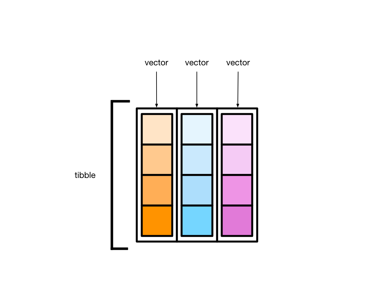
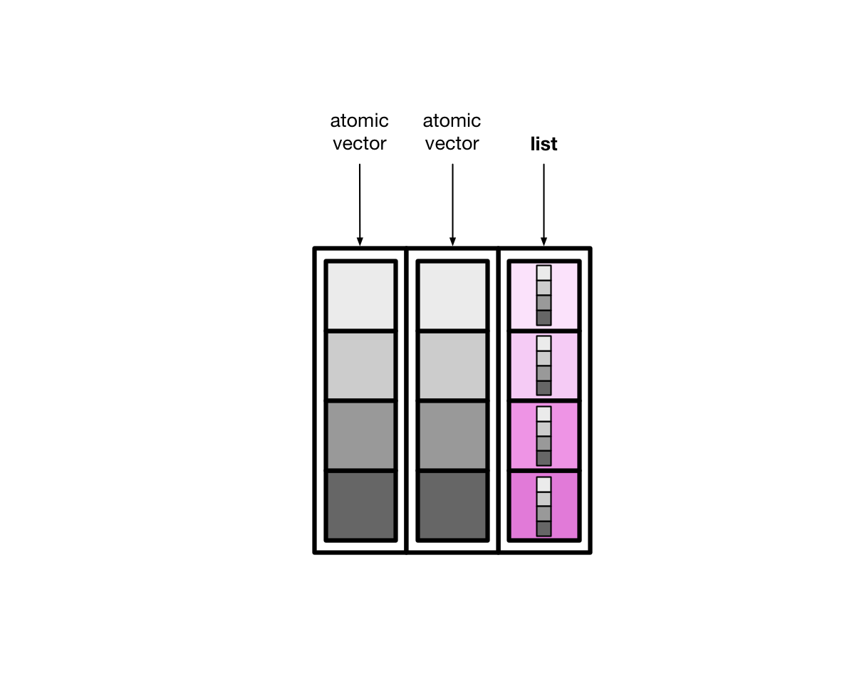
tibble 本质上是向量构成的列表
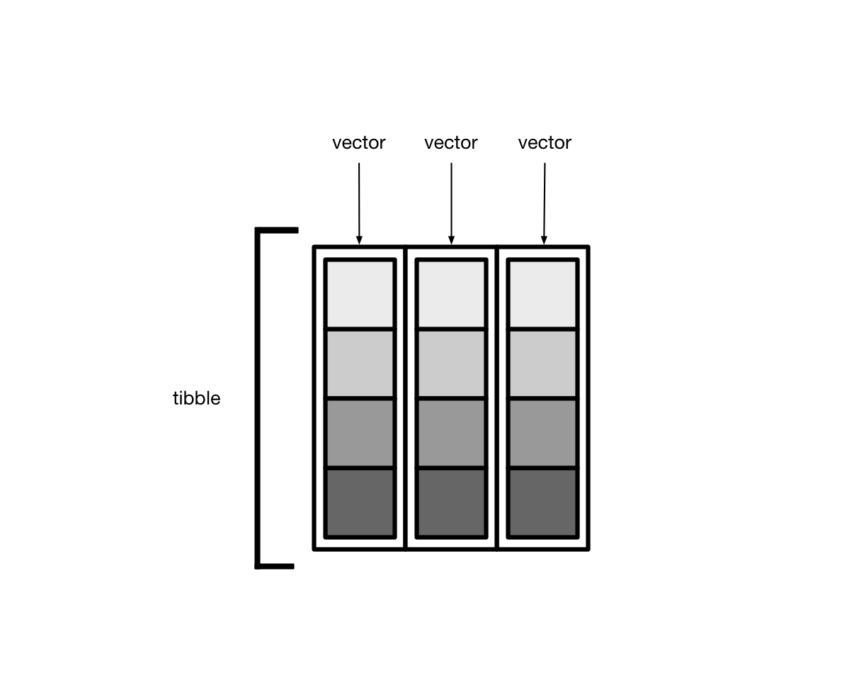
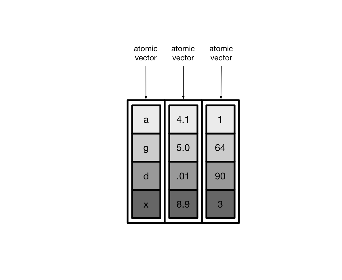
大多情况下,我们接触到的向量是原子型向量(atomic vectors),所谓原子型向量就是向量元素为单个值,比如 “a” 或者 1
tibble还有可以允许某一列为列表(list),那么列表构成的列,称之为列表列(list columns)
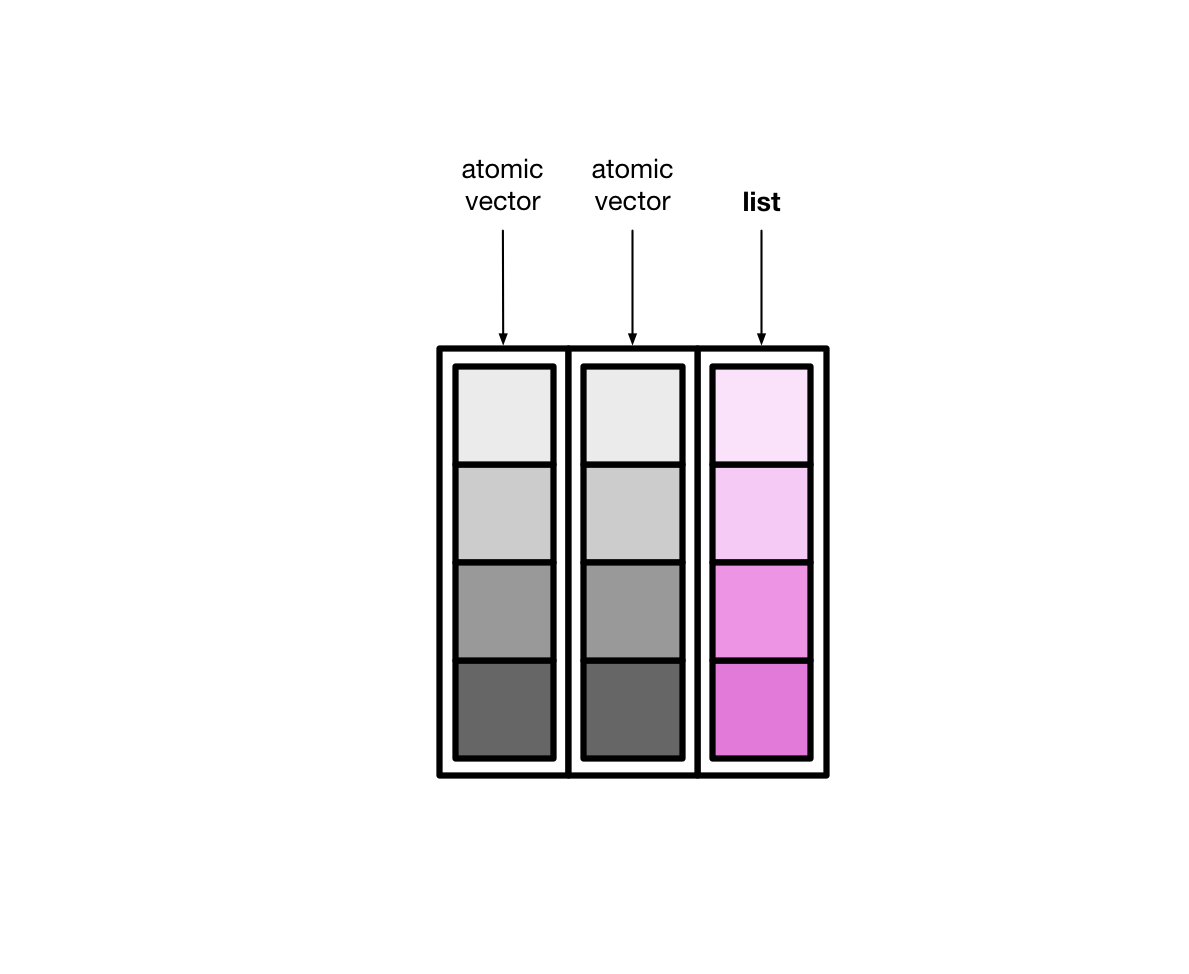
这样一来,列表列非常灵活,因为列表元素可以是原子型向量、列表、矩阵或者小的tibble
nested tibble#
tibble的列表列装载数据的能力很强大,也很灵活。
如何创建和操控有列表列的tibble。
1 creating#
假定我们这里有一个tibble, 我们有三种方法可以创建列表列
nest()summarise()andlist()mutate()andmap()tidyr::nest()创建
使用tidyr::nest(data = c())函数,创建有列表列的tibble, data指定那几列合成列表列data。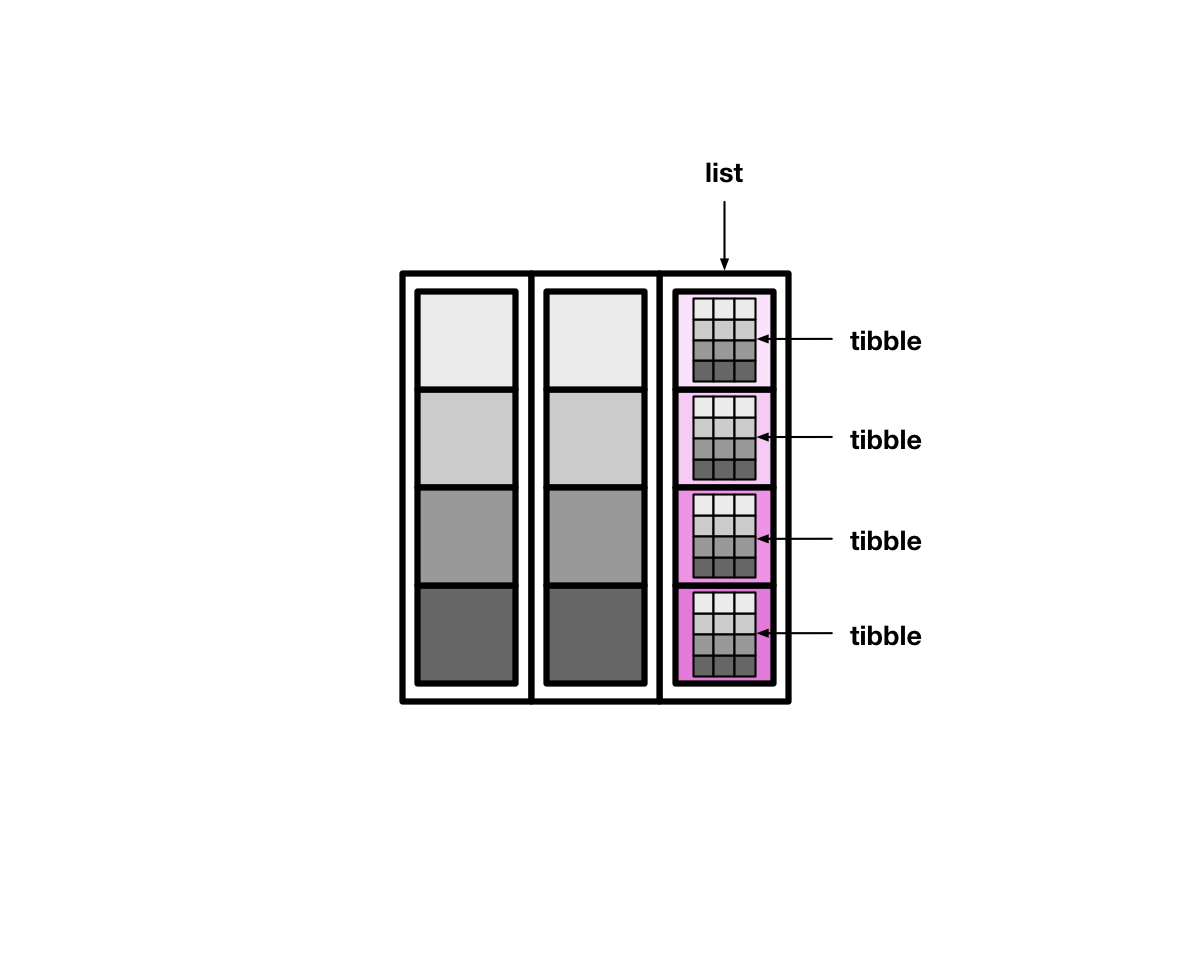
除了x列外的其他列就可用nest(data = !x)
# tidyr::nest()
library(tidyverse)
library(palmerpenguins)
df <- penguins %>%
  drop_na() %>%
  select(species, bill_length_mm, bill_depth_mm, body_mass_g)
df %>% head()

tb <- df %>%
  tidyr::nest(data = c(bill_length_mm, bill_depth_mm, body_mass_g))
tb %>% head()
| species | bill_length_mm | bill_depth_mm | body_mass_g |
|---|---|---|---|
| <fct> | <dbl> | <dbl> | <int> |
| Adelie | 39.1 | 18.7 | 3750 |
| Adelie | 39.5 | 17.4 | 3800 |
| Adelie | 40.3 | 18.0 | 3250 |
| Adelie | 36.7 | 19.3 | 3450 |
| Adelie | 39.3 | 20.6 | 3650 |
| Adelie | 38.9 | 17.8 | 3625 |
| species | data |
|---|---|
| <fct> | <list> |
| Adelie | 39.1, 39.5, 40.3, 36.7, 39.3, 38.9, 39.2, 41.1, 38.6, 34.6, 36.6, 38.7, 42.5, 34.4, 46.0, 37.8, 37.7, 35.9, 38.2, 38.8, 35.3, 40.6, 40.5, 37.9, 40.5, 39.5, 37.2, 39.5, 40.9, 36.4, 39.2, 38.8, 42.2, 37.6, 39.8, 36.5, 40.8, 36.0, 44.1, 37.0, 39.6, 41.1, 36.0, 42.3, 39.6, 40.1, 35.0, 42.0, 34.5, 41.4, 39.0, 40.6, 36.5, 37.6, 35.7, 41.3, 37.6, 41.1, 36.4, 41.6, 35.5, 41.1, 35.9, 41.8, 33.5, 39.7, 39.6, 45.8, 35.5, 42.8, 40.9, 37.2, 36.2, 42.1, 34.6, 42.9, 36.7, 35.1, 37.3, 41.3, 36.3, 36.9, 38.3, 38.9, 35.7, 41.1, 34.0, 39.6, 36.2, 40.8, 38.1, 40.3, 33.1, 43.2, 35.0, 41.0, 37.7, 37.8, 37.9, 39.7, 38.6, 38.2, 38.1, 43.2, 38.1, 45.6, 39.7, 42.2, 39.6, 42.7, 38.6, 37.3, 35.7, 41.1, 36.2, 37.7, 40.2, 41.4, 35.2, 40.6, 38.8, 41.5, 39.0, 44.1, 38.5, 43.1, 36.8, 37.5, 38.1, 41.1, 35.6, 40.2, 37.0, 39.7, 40.2, 40.6, 32.1, 40.7, 37.3, 39.0, 39.2, 36.6, 36.0, 37.8, 36.0, 41.5, 18.7, 17.4, 18.0, 19.3, 20.6, 17.8, 19.6, 17.6, 21.2, 21.1, 17.8, 19.0, 20.7, 18.4, 21.5, 18.3, 18.7, 19.2, 18.1, 17.2, 18.9, 18.6, 17.9, 18.6, 18.9, 16.7, 18.1, 17.8, 18.9, 17.0, 21.1, 20.0, 18.5, 19.3, 19.1, 18.0, 18.4, 18.5, 19.7, 16.9, 18.8, 19.0, 17.9, 21.2, 17.7, 18.9, 17.9, 19.5, 18.1, 18.6, 17.5, 18.8, 16.6, 19.1, 16.9, 21.1, 17.0, 18.2, 17.1, 18.0, 16.2, 19.1, 16.6, 19.4, 19.0, 18.4, 17.2, 18.9, 17.5, 18.5, 16.8, 19.4, 16.1, 19.1, 17.2, 17.6, 18.8, 19.4, 17.8, 20.3, 19.5, 18.6, 19.2, 18.8, 18.0, 18.1, 17.1, 18.1, 17.3, 18.9, 18.6, 18.5, 16.1, 18.5, 17.9, 20.0, 16.0, 20.0, 18.6, 18.9, 17.2, 20.0, 17.0, 19.0, 16.5, 20.3, 17.7, 19.5, 20.7, 18.3, 17.0, 20.5, 17.0, 18.6, 17.2, 19.8, 17.0, 18.5, 15.9, 19.0, 17.6, 18.3, 17.1, 18.0, 17.9, 19.2, 18.5, 18.5, 17.6, 17.5, 17.5, 20.1, 16.5, 17.9, 17.1, 17.2, 15.5, 17.0, 16.8, 18.7, 18.6, 18.4, 17.8, 18.1, 17.1, 18.5, 3750.0, 3800.0, 3250.0, 3450.0, 3650.0, 3625.0, 4675.0, 3200.0, 3800.0, 4400.0, 3700.0, 3450.0, 4500.0, 3325.0, 4200.0, 3400.0, 3600.0, 3800.0, 3950.0, 3800.0, 3800.0, 3550.0, 3200.0, 3150.0, 3950.0, 3250.0, 3900.0, 3300.0, 3900.0, 3325.0, 4150.0, 3950.0, 3550.0, 3300.0, 4650.0, 3150.0, 3900.0, 3100.0, 4400.0, 3000.0, 4600.0, 3425.0, 3450.0, 4150.0, 3500.0, 4300.0, 3450.0, 4050.0, 2900.0, 3700.0, 3550.0, 3800.0, 2850.0, 3750.0, 3150.0, 4400.0, 3600.0, 4050.0, 2850.0, 3950.0, 3350.0, 4100.0, 3050.0, 4450.0, 3600.0, 3900.0, 3550.0, 4150.0, 3700.0, 4250.0, 3700.0, 3900.0, 3550.0, 4000.0, 3200.0, 4700.0, 3800.0, 4200.0, 3350.0, 3550.0, 3800.0, 3500.0, 3950.0, 3600.0, 3550.0, 4300.0, 3400.0, 4450.0, 3300.0, 4300.0, 3700.0, 4350.0, 2900.0, 4100.0, 3725.0, 4725.0, 3075.0, 4250.0, 2925.0, 3550.0, 3750.0, 3900.0, 3175.0, 4775.0, 3825.0, 4600.0, 3200.0, 4275.0, 3900.0, 4075.0, 2900.0, 3775.0, 3350.0, 3325.0, 3150.0, 3500.0, 3450.0, 3875.0, 3050.0, 4000.0, 3275.0, 4300.0, 3050.0, 4000.0, 3325.0, 3500.0, 3500.0, 4475.0, 3425.0, 3900.0, 3175.0, 3975.0, 3400.0, 4250.0, 3400.0, 3475.0, 3050.0, 3725.0, 3000.0, 3650.0, 4250.0, 3475.0, 3450.0, 3750.0, 3700.0, 4000.0 |
| Gentoo | 46.1, 50.0, 48.7, 50.0, 47.6, 46.5, 45.4, 46.7, 43.3, 46.8, 40.9, 49.0, 45.5, 48.4, 45.8, 49.3, 42.0, 49.2, 46.2, 48.7, 50.2, 45.1, 46.5, 46.3, 42.9, 46.1, 47.8, 48.2, 50.0, 47.3, 42.8, 45.1, 59.6, 49.1, 48.4, 42.6, 44.4, 44.0, 48.7, 42.7, 49.6, 45.3, 49.6, 50.5, 43.6, 45.5, 50.5, 44.9, 45.2, 46.6, 48.5, 45.1, 50.1, 46.5, 45.0, 43.8, 45.5, 43.2, 50.4, 45.3, 46.2, 45.7, 54.3, 45.8, 49.8, 49.5, 43.5, 50.7, 47.7, 46.4, 48.2, 46.5, 46.4, 48.6, 47.5, 51.1, 45.2, 45.2, 49.1, 52.5, 47.4, 50.0, 44.9, 50.8, 43.4, 51.3, 47.5, 52.1, 47.5, 52.2, 45.5, 49.5, 44.5, 50.8, 49.4, 46.9, 48.4, 51.1, 48.5, 55.9, 47.2, 49.1, 46.8, 41.7, 53.4, 43.3, 48.1, 50.5, 49.8, 43.5, 51.5, 46.2, 55.1, 48.8, 47.2, 46.8, 50.4, 45.2, 49.9, 13.2, 16.3, 14.1, 15.2, 14.5, 13.5, 14.6, 15.3, 13.4, 15.4, 13.7, 16.1, 13.7, 14.6, 14.6, 15.7, 13.5, 15.2, 14.5, 15.1, 14.3, 14.5, 14.5, 15.8, 13.1, 15.1, 15.0, 14.3, 15.3, 15.3, 14.2, 14.5, 17.0, 14.8, 16.3, 13.7, 17.3, 13.6, 15.7, 13.7, 16.0, 13.7, 15.0, 15.9, 13.9, 13.9, 15.9, 13.3, 15.8, 14.2, 14.1, 14.4, 15.0, 14.4, 15.4, 13.9, 15.0, 14.5, 15.3, 13.8, 14.9, 13.9, 15.7, 14.2, 16.8, 16.2, 14.2, 15.0, 15.0, 15.6, 15.6, 14.8, 15.0, 16.0, 14.2, 16.3, 13.8, 16.4, 14.5, 15.6, 14.6, 15.9, 13.8, 17.3, 14.4, 14.2, 14.0, 17.0, 15.0, 17.1, 14.5, 16.1, 14.7, 15.7, 15.8, 14.6, 14.4, 16.5, 15.0, 17.0, 15.5, 15.0, 16.1, 14.7, 15.8, 14.0, 15.1, 15.2, 15.9, 15.2, 16.3, 14.1, 16.0, 16.2, 13.7, 14.3, 15.7, 14.8, 16.1, 4500.0, 5700.0, 4450.0, 5700.0, 5400.0, 4550.0, 4800.0, 5200.0, 4400.0, 5150.0, 4650.0, 5550.0, 4650.0, 5850.0, 4200.0, 5850.0, 4150.0, 6300.0, 4800.0, 5350.0, 5700.0, 5000.0, 4400.0, 5050.0, 5000.0, 5100.0, 5650.0, 4600.0, 5550.0, 5250.0, 4700.0, 5050.0, 6050.0, 5150.0, 5400.0, 4950.0, 5250.0, 4350.0, 5350.0, 3950.0, 5700.0, 4300.0, 4750.0, 5550.0, 4900.0, 4200.0, 5400.0, 5100.0, 5300.0, 4850.0, 5300.0, 4400.0, 5000.0, 4900.0, 5050.0, 4300.0, 5000.0, 4450.0, 5550.0, 4200.0, 5300.0, 4400.0, 5650.0, 4700.0, 5700.0, 5800.0, 4700.0, 5550.0, 4750.0, 5000.0, 5100.0, 5200.0, 4700.0, 5800.0, 4600.0, 6000.0, 4750.0, 5950.0, 4625.0, 5450.0, 4725.0, 5350.0, 4750.0, 5600.0, 4600.0, 5300.0, 4875.0, 5550.0, 4950.0, 5400.0, 4750.0, 5650.0, 4850.0, 5200.0, 4925.0, 4875.0, 4625.0, 5250.0, 4850.0, 5600.0, 4975.0, 5500.0, 5500.0, 4700.0, 5500.0, 4575.0, 5500.0, 5000.0, 5950.0, 4650.0, 5500.0, 4375.0, 5850.0, 6000.0, 4925.0, 4850.0, 5750.0, 5200.0, 5400.0 |
| Chinstrap | 46.5, 50.0, 51.3, 45.4, 52.7, 45.2, 46.1, 51.3, 46.0, 51.3, 46.6, 51.7, 47.0, 52.0, 45.9, 50.5, 50.3, 58.0, 46.4, 49.2, 42.4, 48.5, 43.2, 50.6, 46.7, 52.0, 50.5, 49.5, 46.4, 52.8, 40.9, 54.2, 42.5, 51.0, 49.7, 47.5, 47.6, 52.0, 46.9, 53.5, 49.0, 46.2, 50.9, 45.5, 50.9, 50.8, 50.1, 49.0, 51.5, 49.8, 48.1, 51.4, 45.7, 50.7, 42.5, 52.2, 45.2, 49.3, 50.2, 45.6, 51.9, 46.8, 45.7, 55.8, 43.5, 49.6, 50.8, 50.2, 17.9, 19.5, 19.2, 18.7, 19.8, 17.8, 18.2, 18.2, 18.9, 19.9, 17.8, 20.3, 17.3, 18.1, 17.1, 19.6, 20.0, 17.8, 18.6, 18.2, 17.3, 17.5, 16.6, 19.4, 17.9, 19.0, 18.4, 19.0, 17.8, 20.0, 16.6, 20.8, 16.7, 18.8, 18.6, 16.8, 18.3, 20.7, 16.6, 19.9, 19.5, 17.5, 19.1, 17.0, 17.9, 18.5, 17.9, 19.6, 18.7, 17.3, 16.4, 19.0, 17.3, 19.7, 17.3, 18.8, 16.6, 19.9, 18.8, 19.4, 19.5, 16.5, 17.0, 19.8, 18.1, 18.2, 19.0, 18.7, 3500.0, 3900.0, 3650.0, 3525.0, 3725.0, 3950.0, 3250.0, 3750.0, 4150.0, 3700.0, 3800.0, 3775.0, 3700.0, 4050.0, 3575.0, 4050.0, 3300.0, 3700.0, 3450.0, 4400.0, 3600.0, 3400.0, 2900.0, 3800.0, 3300.0, 4150.0, 3400.0, 3800.0, 3700.0, 4550.0, 3200.0, 4300.0, 3350.0, 4100.0, 3600.0, 3900.0, 3850.0, 4800.0, 2700.0, 4500.0, 3950.0, 3650.0, 3550.0, 3500.0, 3675.0, 4450.0, 3400.0, 4300.0, 3250.0, 3675.0, 3325.0, 3950.0, 3600.0, 4050.0, 3350.0, 3450.0, 3250.0, 4050.0, 3800.0, 3525.0, 3950.0, 3650.0, 3650.0, 4000.0, 3400.0, 3775.0, 4100.0, 3775.0 |
nest() 为每种species创建了一个小的tibble, 每个小的tibble对应一个species
tb$data[[1]] %>% head()
tb$data %>% typeof()
tb$data %>% class()
| bill_length_mm | bill_depth_mm | body_mass_g |
|---|---|---|
| <dbl> | <dbl> | <int> |
| 39.1 | 18.7 | 3750 |
| 39.5 | 17.4 | 3800 |
| 40.3 | 18.0 | 3250 |
| 36.7 | 19.3 | 3450 |
| 39.3 | 20.6 | 3650 |
| 38.9 | 17.8 | 3625 |
# 除了species列之外的其他列组合成list_columns
df %>%
  nest(data = !species)
| species | data |
|---|---|
| <fct> | <list> |
| Adelie | 39.1, 39.5, 40.3, 36.7, 39.3, 38.9, 39.2, 41.1, 38.6, 34.6, 36.6, 38.7, 42.5, 34.4, 46.0, 37.8, 37.7, 35.9, 38.2, 38.8, 35.3, 40.6, 40.5, 37.9, 40.5, 39.5, 37.2, 39.5, 40.9, 36.4, 39.2, 38.8, 42.2, 37.6, 39.8, 36.5, 40.8, 36.0, 44.1, 37.0, 39.6, 41.1, 36.0, 42.3, 39.6, 40.1, 35.0, 42.0, 34.5, 41.4, 39.0, 40.6, 36.5, 37.6, 35.7, 41.3, 37.6, 41.1, 36.4, 41.6, 35.5, 41.1, 35.9, 41.8, 33.5, 39.7, 39.6, 45.8, 35.5, 42.8, 40.9, 37.2, 36.2, 42.1, 34.6, 42.9, 36.7, 35.1, 37.3, 41.3, 36.3, 36.9, 38.3, 38.9, 35.7, 41.1, 34.0, 39.6, 36.2, 40.8, 38.1, 40.3, 33.1, 43.2, 35.0, 41.0, 37.7, 37.8, 37.9, 39.7, 38.6, 38.2, 38.1, 43.2, 38.1, 45.6, 39.7, 42.2, 39.6, 42.7, 38.6, 37.3, 35.7, 41.1, 36.2, 37.7, 40.2, 41.4, 35.2, 40.6, 38.8, 41.5, 39.0, 44.1, 38.5, 43.1, 36.8, 37.5, 38.1, 41.1, 35.6, 40.2, 37.0, 39.7, 40.2, 40.6, 32.1, 40.7, 37.3, 39.0, 39.2, 36.6, 36.0, 37.8, 36.0, 41.5, 18.7, 17.4, 18.0, 19.3, 20.6, 17.8, 19.6, 17.6, 21.2, 21.1, 17.8, 19.0, 20.7, 18.4, 21.5, 18.3, 18.7, 19.2, 18.1, 17.2, 18.9, 18.6, 17.9, 18.6, 18.9, 16.7, 18.1, 17.8, 18.9, 17.0, 21.1, 20.0, 18.5, 19.3, 19.1, 18.0, 18.4, 18.5, 19.7, 16.9, 18.8, 19.0, 17.9, 21.2, 17.7, 18.9, 17.9, 19.5, 18.1, 18.6, 17.5, 18.8, 16.6, 19.1, 16.9, 21.1, 17.0, 18.2, 17.1, 18.0, 16.2, 19.1, 16.6, 19.4, 19.0, 18.4, 17.2, 18.9, 17.5, 18.5, 16.8, 19.4, 16.1, 19.1, 17.2, 17.6, 18.8, 19.4, 17.8, 20.3, 19.5, 18.6, 19.2, 18.8, 18.0, 18.1, 17.1, 18.1, 17.3, 18.9, 18.6, 18.5, 16.1, 18.5, 17.9, 20.0, 16.0, 20.0, 18.6, 18.9, 17.2, 20.0, 17.0, 19.0, 16.5, 20.3, 17.7, 19.5, 20.7, 18.3, 17.0, 20.5, 17.0, 18.6, 17.2, 19.8, 17.0, 18.5, 15.9, 19.0, 17.6, 18.3, 17.1, 18.0, 17.9, 19.2, 18.5, 18.5, 17.6, 17.5, 17.5, 20.1, 16.5, 17.9, 17.1, 17.2, 15.5, 17.0, 16.8, 18.7, 18.6, 18.4, 17.8, 18.1, 17.1, 18.5, 3750.0, 3800.0, 3250.0, 3450.0, 3650.0, 3625.0, 4675.0, 3200.0, 3800.0, 4400.0, 3700.0, 3450.0, 4500.0, 3325.0, 4200.0, 3400.0, 3600.0, 3800.0, 3950.0, 3800.0, 3800.0, 3550.0, 3200.0, 3150.0, 3950.0, 3250.0, 3900.0, 3300.0, 3900.0, 3325.0, 4150.0, 3950.0, 3550.0, 3300.0, 4650.0, 3150.0, 3900.0, 3100.0, 4400.0, 3000.0, 4600.0, 3425.0, 3450.0, 4150.0, 3500.0, 4300.0, 3450.0, 4050.0, 2900.0, 3700.0, 3550.0, 3800.0, 2850.0, 3750.0, 3150.0, 4400.0, 3600.0, 4050.0, 2850.0, 3950.0, 3350.0, 4100.0, 3050.0, 4450.0, 3600.0, 3900.0, 3550.0, 4150.0, 3700.0, 4250.0, 3700.0, 3900.0, 3550.0, 4000.0, 3200.0, 4700.0, 3800.0, 4200.0, 3350.0, 3550.0, 3800.0, 3500.0, 3950.0, 3600.0, 3550.0, 4300.0, 3400.0, 4450.0, 3300.0, 4300.0, 3700.0, 4350.0, 2900.0, 4100.0, 3725.0, 4725.0, 3075.0, 4250.0, 2925.0, 3550.0, 3750.0, 3900.0, 3175.0, 4775.0, 3825.0, 4600.0, 3200.0, 4275.0, 3900.0, 4075.0, 2900.0, 3775.0, 3350.0, 3325.0, 3150.0, 3500.0, 3450.0, 3875.0, 3050.0, 4000.0, 3275.0, 4300.0, 3050.0, 4000.0, 3325.0, 3500.0, 3500.0, 4475.0, 3425.0, 3900.0, 3175.0, 3975.0, 3400.0, 4250.0, 3400.0, 3475.0, 3050.0, 3725.0, 3000.0, 3650.0, 4250.0, 3475.0, 3450.0, 3750.0, 3700.0, 4000.0 |
| Gentoo | 46.1, 50.0, 48.7, 50.0, 47.6, 46.5, 45.4, 46.7, 43.3, 46.8, 40.9, 49.0, 45.5, 48.4, 45.8, 49.3, 42.0, 49.2, 46.2, 48.7, 50.2, 45.1, 46.5, 46.3, 42.9, 46.1, 47.8, 48.2, 50.0, 47.3, 42.8, 45.1, 59.6, 49.1, 48.4, 42.6, 44.4, 44.0, 48.7, 42.7, 49.6, 45.3, 49.6, 50.5, 43.6, 45.5, 50.5, 44.9, 45.2, 46.6, 48.5, 45.1, 50.1, 46.5, 45.0, 43.8, 45.5, 43.2, 50.4, 45.3, 46.2, 45.7, 54.3, 45.8, 49.8, 49.5, 43.5, 50.7, 47.7, 46.4, 48.2, 46.5, 46.4, 48.6, 47.5, 51.1, 45.2, 45.2, 49.1, 52.5, 47.4, 50.0, 44.9, 50.8, 43.4, 51.3, 47.5, 52.1, 47.5, 52.2, 45.5, 49.5, 44.5, 50.8, 49.4, 46.9, 48.4, 51.1, 48.5, 55.9, 47.2, 49.1, 46.8, 41.7, 53.4, 43.3, 48.1, 50.5, 49.8, 43.5, 51.5, 46.2, 55.1, 48.8, 47.2, 46.8, 50.4, 45.2, 49.9, 13.2, 16.3, 14.1, 15.2, 14.5, 13.5, 14.6, 15.3, 13.4, 15.4, 13.7, 16.1, 13.7, 14.6, 14.6, 15.7, 13.5, 15.2, 14.5, 15.1, 14.3, 14.5, 14.5, 15.8, 13.1, 15.1, 15.0, 14.3, 15.3, 15.3, 14.2, 14.5, 17.0, 14.8, 16.3, 13.7, 17.3, 13.6, 15.7, 13.7, 16.0, 13.7, 15.0, 15.9, 13.9, 13.9, 15.9, 13.3, 15.8, 14.2, 14.1, 14.4, 15.0, 14.4, 15.4, 13.9, 15.0, 14.5, 15.3, 13.8, 14.9, 13.9, 15.7, 14.2, 16.8, 16.2, 14.2, 15.0, 15.0, 15.6, 15.6, 14.8, 15.0, 16.0, 14.2, 16.3, 13.8, 16.4, 14.5, 15.6, 14.6, 15.9, 13.8, 17.3, 14.4, 14.2, 14.0, 17.0, 15.0, 17.1, 14.5, 16.1, 14.7, 15.7, 15.8, 14.6, 14.4, 16.5, 15.0, 17.0, 15.5, 15.0, 16.1, 14.7, 15.8, 14.0, 15.1, 15.2, 15.9, 15.2, 16.3, 14.1, 16.0, 16.2, 13.7, 14.3, 15.7, 14.8, 16.1, 4500.0, 5700.0, 4450.0, 5700.0, 5400.0, 4550.0, 4800.0, 5200.0, 4400.0, 5150.0, 4650.0, 5550.0, 4650.0, 5850.0, 4200.0, 5850.0, 4150.0, 6300.0, 4800.0, 5350.0, 5700.0, 5000.0, 4400.0, 5050.0, 5000.0, 5100.0, 5650.0, 4600.0, 5550.0, 5250.0, 4700.0, 5050.0, 6050.0, 5150.0, 5400.0, 4950.0, 5250.0, 4350.0, 5350.0, 3950.0, 5700.0, 4300.0, 4750.0, 5550.0, 4900.0, 4200.0, 5400.0, 5100.0, 5300.0, 4850.0, 5300.0, 4400.0, 5000.0, 4900.0, 5050.0, 4300.0, 5000.0, 4450.0, 5550.0, 4200.0, 5300.0, 4400.0, 5650.0, 4700.0, 5700.0, 5800.0, 4700.0, 5550.0, 4750.0, 5000.0, 5100.0, 5200.0, 4700.0, 5800.0, 4600.0, 6000.0, 4750.0, 5950.0, 4625.0, 5450.0, 4725.0, 5350.0, 4750.0, 5600.0, 4600.0, 5300.0, 4875.0, 5550.0, 4950.0, 5400.0, 4750.0, 5650.0, 4850.0, 5200.0, 4925.0, 4875.0, 4625.0, 5250.0, 4850.0, 5600.0, 4975.0, 5500.0, 5500.0, 4700.0, 5500.0, 4575.0, 5500.0, 5000.0, 5950.0, 4650.0, 5500.0, 4375.0, 5850.0, 6000.0, 4925.0, 4850.0, 5750.0, 5200.0, 5400.0 |
| Chinstrap | 46.5, 50.0, 51.3, 45.4, 52.7, 45.2, 46.1, 51.3, 46.0, 51.3, 46.6, 51.7, 47.0, 52.0, 45.9, 50.5, 50.3, 58.0, 46.4, 49.2, 42.4, 48.5, 43.2, 50.6, 46.7, 52.0, 50.5, 49.5, 46.4, 52.8, 40.9, 54.2, 42.5, 51.0, 49.7, 47.5, 47.6, 52.0, 46.9, 53.5, 49.0, 46.2, 50.9, 45.5, 50.9, 50.8, 50.1, 49.0, 51.5, 49.8, 48.1, 51.4, 45.7, 50.7, 42.5, 52.2, 45.2, 49.3, 50.2, 45.6, 51.9, 46.8, 45.7, 55.8, 43.5, 49.6, 50.8, 50.2, 17.9, 19.5, 19.2, 18.7, 19.8, 17.8, 18.2, 18.2, 18.9, 19.9, 17.8, 20.3, 17.3, 18.1, 17.1, 19.6, 20.0, 17.8, 18.6, 18.2, 17.3, 17.5, 16.6, 19.4, 17.9, 19.0, 18.4, 19.0, 17.8, 20.0, 16.6, 20.8, 16.7, 18.8, 18.6, 16.8, 18.3, 20.7, 16.6, 19.9, 19.5, 17.5, 19.1, 17.0, 17.9, 18.5, 17.9, 19.6, 18.7, 17.3, 16.4, 19.0, 17.3, 19.7, 17.3, 18.8, 16.6, 19.9, 18.8, 19.4, 19.5, 16.5, 17.0, 19.8, 18.1, 18.2, 19.0, 18.7, 3500.0, 3900.0, 3650.0, 3525.0, 3725.0, 3950.0, 3250.0, 3750.0, 4150.0, 3700.0, 3800.0, 3775.0, 3700.0, 4050.0, 3575.0, 4050.0, 3300.0, 3700.0, 3450.0, 4400.0, 3600.0, 3400.0, 2900.0, 3800.0, 3300.0, 4150.0, 3400.0, 3800.0, 3700.0, 4550.0, 3200.0, 4300.0, 3350.0, 4100.0, 3600.0, 3900.0, 3850.0, 4800.0, 2700.0, 4500.0, 3950.0, 3650.0, 3550.0, 3500.0, 3675.0, 4450.0, 3400.0, 4300.0, 3250.0, 3675.0, 3325.0, 3950.0, 3600.0, 4050.0, 3350.0, 3450.0, 3250.0, 4050.0, 3800.0, 3525.0, 3950.0, 3650.0, 3650.0, 4000.0, 3400.0, 3775.0, 4100.0, 3775.0 |
# 同时创建多个列表列
df %>%
  nest(data1 = c(bill_length_mm, bill_depth_mm), data2 = body_mass_g)
| species | data1 | data2 |
|---|---|---|
| <fct> | <list> | <list> |
| Adelie | 39.1, 39.5, 40.3, 36.7, 39.3, 38.9, 39.2, 41.1, 38.6, 34.6, 36.6, 38.7, 42.5, 34.4, 46.0, 37.8, 37.7, 35.9, 38.2, 38.8, 35.3, 40.6, 40.5, 37.9, 40.5, 39.5, 37.2, 39.5, 40.9, 36.4, 39.2, 38.8, 42.2, 37.6, 39.8, 36.5, 40.8, 36.0, 44.1, 37.0, 39.6, 41.1, 36.0, 42.3, 39.6, 40.1, 35.0, 42.0, 34.5, 41.4, 39.0, 40.6, 36.5, 37.6, 35.7, 41.3, 37.6, 41.1, 36.4, 41.6, 35.5, 41.1, 35.9, 41.8, 33.5, 39.7, 39.6, 45.8, 35.5, 42.8, 40.9, 37.2, 36.2, 42.1, 34.6, 42.9, 36.7, 35.1, 37.3, 41.3, 36.3, 36.9, 38.3, 38.9, 35.7, 41.1, 34.0, 39.6, 36.2, 40.8, 38.1, 40.3, 33.1, 43.2, 35.0, 41.0, 37.7, 37.8, 37.9, 39.7, 38.6, 38.2, 38.1, 43.2, 38.1, 45.6, 39.7, 42.2, 39.6, 42.7, 38.6, 37.3, 35.7, 41.1, 36.2, 37.7, 40.2, 41.4, 35.2, 40.6, 38.8, 41.5, 39.0, 44.1, 38.5, 43.1, 36.8, 37.5, 38.1, 41.1, 35.6, 40.2, 37.0, 39.7, 40.2, 40.6, 32.1, 40.7, 37.3, 39.0, 39.2, 36.6, 36.0, 37.8, 36.0, 41.5, 18.7, 17.4, 18.0, 19.3, 20.6, 17.8, 19.6, 17.6, 21.2, 21.1, 17.8, 19.0, 20.7, 18.4, 21.5, 18.3, 18.7, 19.2, 18.1, 17.2, 18.9, 18.6, 17.9, 18.6, 18.9, 16.7, 18.1, 17.8, 18.9, 17.0, 21.1, 20.0, 18.5, 19.3, 19.1, 18.0, 18.4, 18.5, 19.7, 16.9, 18.8, 19.0, 17.9, 21.2, 17.7, 18.9, 17.9, 19.5, 18.1, 18.6, 17.5, 18.8, 16.6, 19.1, 16.9, 21.1, 17.0, 18.2, 17.1, 18.0, 16.2, 19.1, 16.6, 19.4, 19.0, 18.4, 17.2, 18.9, 17.5, 18.5, 16.8, 19.4, 16.1, 19.1, 17.2, 17.6, 18.8, 19.4, 17.8, 20.3, 19.5, 18.6, 19.2, 18.8, 18.0, 18.1, 17.1, 18.1, 17.3, 18.9, 18.6, 18.5, 16.1, 18.5, 17.9, 20.0, 16.0, 20.0, 18.6, 18.9, 17.2, 20.0, 17.0, 19.0, 16.5, 20.3, 17.7, 19.5, 20.7, 18.3, 17.0, 20.5, 17.0, 18.6, 17.2, 19.8, 17.0, 18.5, 15.9, 19.0, 17.6, 18.3, 17.1, 18.0, 17.9, 19.2, 18.5, 18.5, 17.6, 17.5, 17.5, 20.1, 16.5, 17.9, 17.1, 17.2, 15.5, 17.0, 16.8, 18.7, 18.6, 18.4, 17.8, 18.1, 17.1, 18.5 | 3750, 3800, 3250, 3450, 3650, 3625, 4675, 3200, 3800, 4400, 3700, 3450, 4500, 3325, 4200, 3400, 3600, 3800, 3950, 3800, 3800, 3550, 3200, 3150, 3950, 3250, 3900, 3300, 3900, 3325, 4150, 3950, 3550, 3300, 4650, 3150, 3900, 3100, 4400, 3000, 4600, 3425, 3450, 4150, 3500, 4300, 3450, 4050, 2900, 3700, 3550, 3800, 2850, 3750, 3150, 4400, 3600, 4050, 2850, 3950, 3350, 4100, 3050, 4450, 3600, 3900, 3550, 4150, 3700, 4250, 3700, 3900, 3550, 4000, 3200, 4700, 3800, 4200, 3350, 3550, 3800, 3500, 3950, 3600, 3550, 4300, 3400, 4450, 3300, 4300, 3700, 4350, 2900, 4100, 3725, 4725, 3075, 4250, 2925, 3550, 3750, 3900, 3175, 4775, 3825, 4600, 3200, 4275, 3900, 4075, 2900, 3775, 3350, 3325, 3150, 3500, 3450, 3875, 3050, 4000, 3275, 4300, 3050, 4000, 3325, 3500, 3500, 4475, 3425, 3900, 3175, 3975, 3400, 4250, 3400, 3475, 3050, 3725, 3000, 3650, 4250, 3475, 3450, 3750, 3700, 4000 |
| Gentoo | 46.1, 50.0, 48.7, 50.0, 47.6, 46.5, 45.4, 46.7, 43.3, 46.8, 40.9, 49.0, 45.5, 48.4, 45.8, 49.3, 42.0, 49.2, 46.2, 48.7, 50.2, 45.1, 46.5, 46.3, 42.9, 46.1, 47.8, 48.2, 50.0, 47.3, 42.8, 45.1, 59.6, 49.1, 48.4, 42.6, 44.4, 44.0, 48.7, 42.7, 49.6, 45.3, 49.6, 50.5, 43.6, 45.5, 50.5, 44.9, 45.2, 46.6, 48.5, 45.1, 50.1, 46.5, 45.0, 43.8, 45.5, 43.2, 50.4, 45.3, 46.2, 45.7, 54.3, 45.8, 49.8, 49.5, 43.5, 50.7, 47.7, 46.4, 48.2, 46.5, 46.4, 48.6, 47.5, 51.1, 45.2, 45.2, 49.1, 52.5, 47.4, 50.0, 44.9, 50.8, 43.4, 51.3, 47.5, 52.1, 47.5, 52.2, 45.5, 49.5, 44.5, 50.8, 49.4, 46.9, 48.4, 51.1, 48.5, 55.9, 47.2, 49.1, 46.8, 41.7, 53.4, 43.3, 48.1, 50.5, 49.8, 43.5, 51.5, 46.2, 55.1, 48.8, 47.2, 46.8, 50.4, 45.2, 49.9, 13.2, 16.3, 14.1, 15.2, 14.5, 13.5, 14.6, 15.3, 13.4, 15.4, 13.7, 16.1, 13.7, 14.6, 14.6, 15.7, 13.5, 15.2, 14.5, 15.1, 14.3, 14.5, 14.5, 15.8, 13.1, 15.1, 15.0, 14.3, 15.3, 15.3, 14.2, 14.5, 17.0, 14.8, 16.3, 13.7, 17.3, 13.6, 15.7, 13.7, 16.0, 13.7, 15.0, 15.9, 13.9, 13.9, 15.9, 13.3, 15.8, 14.2, 14.1, 14.4, 15.0, 14.4, 15.4, 13.9, 15.0, 14.5, 15.3, 13.8, 14.9, 13.9, 15.7, 14.2, 16.8, 16.2, 14.2, 15.0, 15.0, 15.6, 15.6, 14.8, 15.0, 16.0, 14.2, 16.3, 13.8, 16.4, 14.5, 15.6, 14.6, 15.9, 13.8, 17.3, 14.4, 14.2, 14.0, 17.0, 15.0, 17.1, 14.5, 16.1, 14.7, 15.7, 15.8, 14.6, 14.4, 16.5, 15.0, 17.0, 15.5, 15.0, 16.1, 14.7, 15.8, 14.0, 15.1, 15.2, 15.9, 15.2, 16.3, 14.1, 16.0, 16.2, 13.7, 14.3, 15.7, 14.8, 16.1 | 4500, 5700, 4450, 5700, 5400, 4550, 4800, 5200, 4400, 5150, 4650, 5550, 4650, 5850, 4200, 5850, 4150, 6300, 4800, 5350, 5700, 5000, 4400, 5050, 5000, 5100, 5650, 4600, 5550, 5250, 4700, 5050, 6050, 5150, 5400, 4950, 5250, 4350, 5350, 3950, 5700, 4300, 4750, 5550, 4900, 4200, 5400, 5100, 5300, 4850, 5300, 4400, 5000, 4900, 5050, 4300, 5000, 4450, 5550, 4200, 5300, 4400, 5650, 4700, 5700, 5800, 4700, 5550, 4750, 5000, 5100, 5200, 4700, 5800, 4600, 6000, 4750, 5950, 4625, 5450, 4725, 5350, 4750, 5600, 4600, 5300, 4875, 5550, 4950, 5400, 4750, 5650, 4850, 5200, 4925, 4875, 4625, 5250, 4850, 5600, 4975, 5500, 5500, 4700, 5500, 4575, 5500, 5000, 5950, 4650, 5500, 4375, 5850, 6000, 4925, 4850, 5750, 5200, 5400 |
| Chinstrap | 46.5, 50.0, 51.3, 45.4, 52.7, 45.2, 46.1, 51.3, 46.0, 51.3, 46.6, 51.7, 47.0, 52.0, 45.9, 50.5, 50.3, 58.0, 46.4, 49.2, 42.4, 48.5, 43.2, 50.6, 46.7, 52.0, 50.5, 49.5, 46.4, 52.8, 40.9, 54.2, 42.5, 51.0, 49.7, 47.5, 47.6, 52.0, 46.9, 53.5, 49.0, 46.2, 50.9, 45.5, 50.9, 50.8, 50.1, 49.0, 51.5, 49.8, 48.1, 51.4, 45.7, 50.7, 42.5, 52.2, 45.2, 49.3, 50.2, 45.6, 51.9, 46.8, 45.7, 55.8, 43.5, 49.6, 50.8, 50.2, 17.9, 19.5, 19.2, 18.7, 19.8, 17.8, 18.2, 18.2, 18.9, 19.9, 17.8, 20.3, 17.3, 18.1, 17.1, 19.6, 20.0, 17.8, 18.6, 18.2, 17.3, 17.5, 16.6, 19.4, 17.9, 19.0, 18.4, 19.0, 17.8, 20.0, 16.6, 20.8, 16.7, 18.8, 18.6, 16.8, 18.3, 20.7, 16.6, 19.9, 19.5, 17.5, 19.1, 17.0, 17.9, 18.5, 17.9, 19.6, 18.7, 17.3, 16.4, 19.0, 17.3, 19.7, 17.3, 18.8, 16.6, 19.9, 18.8, 19.4, 19.5, 16.5, 17.0, 19.8, 18.1, 18.2, 19.0, 18.7 | 3500, 3900, 3650, 3525, 3725, 3950, 3250, 3750, 4150, 3700, 3800, 3775, 3700, 4050, 3575, 4050, 3300, 3700, 3450, 4400, 3600, 3400, 2900, 3800, 3300, 4150, 3400, 3800, 3700, 4550, 3200, 4300, 3350, 4100, 3600, 3900, 3850, 4800, 2700, 4500, 3950, 3650, 3550, 3500, 3675, 4450, 3400, 4300, 3250, 3675, 3325, 3950, 3600, 4050, 3350, 3450, 3250, 4050, 3800, 3525, 3950, 3650, 3650, 4000, 3400, 3775, 4100, 3775 |
1 creating#
tidyr::summarise(list())创建#
group_by() 和 summarise()组合可以将向量分组后分别压缩成单个值,事实上,summarise()还可以创建列表列。
df_collpase <- df %>%
  group_by(species) %>%
  summarise(data = list(bill_length_mm))
df_collpase
| species | data |
|---|---|
| <fct> | <list> |
| Adelie | 39.1, 39.5, 40.3, 36.7, 39.3, 38.9, 39.2, 41.1, 38.6, 34.6, 36.6, 38.7, 42.5, 34.4, 46.0, 37.8, 37.7, 35.9, 38.2, 38.8, 35.3, 40.6, 40.5, 37.9, 40.5, 39.5, 37.2, 39.5, 40.9, 36.4, 39.2, 38.8, 42.2, 37.6, 39.8, 36.5, 40.8, 36.0, 44.1, 37.0, 39.6, 41.1, 36.0, 42.3, 39.6, 40.1, 35.0, 42.0, 34.5, 41.4, 39.0, 40.6, 36.5, 37.6, 35.7, 41.3, 37.6, 41.1, 36.4, 41.6, 35.5, 41.1, 35.9, 41.8, 33.5, 39.7, 39.6, 45.8, 35.5, 42.8, 40.9, 37.2, 36.2, 42.1, 34.6, 42.9, 36.7, 35.1, 37.3, 41.3, 36.3, 36.9, 38.3, 38.9, 35.7, 41.1, 34.0, 39.6, 36.2, 40.8, 38.1, 40.3, 33.1, 43.2, 35.0, 41.0, 37.7, 37.8, 37.9, 39.7, 38.6, 38.2, 38.1, 43.2, 38.1, 45.6, 39.7, 42.2, 39.6, 42.7, 38.6, 37.3, 35.7, 41.1, 36.2, 37.7, 40.2, 41.4, 35.2, 40.6, 38.8, 41.5, 39.0, 44.1, 38.5, 43.1, 36.8, 37.5, 38.1, 41.1, 35.6, 40.2, 37.0, 39.7, 40.2, 40.6, 32.1, 40.7, 37.3, 39.0, 39.2, 36.6, 36.0, 37.8, 36.0, 41.5 |
| Chinstrap | 46.5, 50.0, 51.3, 45.4, 52.7, 45.2, 46.1, 51.3, 46.0, 51.3, 46.6, 51.7, 47.0, 52.0, 45.9, 50.5, 50.3, 58.0, 46.4, 49.2, 42.4, 48.5, 43.2, 50.6, 46.7, 52.0, 50.5, 49.5, 46.4, 52.8, 40.9, 54.2, 42.5, 51.0, 49.7, 47.5, 47.6, 52.0, 46.9, 53.5, 49.0, 46.2, 50.9, 45.5, 50.9, 50.8, 50.1, 49.0, 51.5, 49.8, 48.1, 51.4, 45.7, 50.7, 42.5, 52.2, 45.2, 49.3, 50.2, 45.6, 51.9, 46.8, 45.7, 55.8, 43.5, 49.6, 50.8, 50.2 |
| Gentoo | 46.1, 50.0, 48.7, 50.0, 47.6, 46.5, 45.4, 46.7, 43.3, 46.8, 40.9, 49.0, 45.5, 48.4, 45.8, 49.3, 42.0, 49.2, 46.2, 48.7, 50.2, 45.1, 46.5, 46.3, 42.9, 46.1, 47.8, 48.2, 50.0, 47.3, 42.8, 45.1, 59.6, 49.1, 48.4, 42.6, 44.4, 44.0, 48.7, 42.7, 49.6, 45.3, 49.6, 50.5, 43.6, 45.5, 50.5, 44.9, 45.2, 46.6, 48.5, 45.1, 50.1, 46.5, 45.0, 43.8, 45.5, 43.2, 50.4, 45.3, 46.2, 45.7, 54.3, 45.8, 49.8, 49.5, 43.5, 50.7, 47.7, 46.4, 48.2, 46.5, 46.4, 48.6, 47.5, 51.1, 45.2, 45.2, 49.1, 52.5, 47.4, 50.0, 44.9, 50.8, 43.4, 51.3, 47.5, 52.1, 47.5, 52.2, 45.5, 49.5, 44.5, 50.8, 49.4, 46.9, 48.4, 51.1, 48.5, 55.9, 47.2, 49.1, 46.8, 41.7, 53.4, 43.3, 48.1, 50.5, 49.8, 43.5, 51.5, 46.2, 55.1, 48.8, 47.2, 46.8, 50.4, 45.2, 49.9 |
data就是构建的列表列,它的每个元素都是一个向量,对应一个species。这种方法和nest()方法很相似,不同在于,summarise() + list() 构建的列表列其元素是原子型向量,而nest()构建的是tibble.
df_collpase$data[[1]] %>% typeof()
summarise() + list()的方法还可以在创建列表列之前,对数据简单处理
# 排序
df %>%
  group_by(species) %>%
  summarise(data = list(sort(bill_length_mm)))

# 筛选
df %>%
  group_by(species) %>%
  summarise(data = list(bill_length_mm[bill_length_mm > 45]))
| species | data |
|---|---|
| <fct> | <list> |
| Adelie | 32.1, 33.1, 33.5, 34.0, 34.4, 34.5, 34.6, 34.6, 35.0, 35.0, 35.1, 35.2, 35.3, 35.5, 35.5, 35.6, 35.7, 35.7, 35.7, 35.9, 35.9, 36.0, 36.0, 36.0, 36.0, 36.2, 36.2, 36.2, 36.3, 36.4, 36.4, 36.5, 36.5, 36.6, 36.6, 36.7, 36.7, 36.8, 36.9, 37.0, 37.0, 37.2, 37.2, 37.3, 37.3, 37.3, 37.5, 37.6, 37.6, 37.6, 37.7, 37.7, 37.7, 37.8, 37.8, 37.8, 37.9, 37.9, 38.1, 38.1, 38.1, 38.1, 38.2, 38.2, 38.3, 38.5, 38.6, 38.6, 38.6, 38.7, 38.8, 38.8, 38.8, 38.9, 38.9, 39.0, 39.0, 39.0, 39.1, 39.2, 39.2, 39.2, 39.3, 39.5, 39.5, 39.5, 39.6, 39.6, 39.6, 39.6, 39.6, 39.7, 39.7, 39.7, 39.7, 39.8, 40.1, 40.2, 40.2, 40.2, 40.3, 40.3, 40.5, 40.5, 40.6, 40.6, 40.6, 40.6, 40.7, 40.8, 40.8, 40.9, 40.9, 41.0, 41.1, 41.1, 41.1, 41.1, 41.1, 41.1, 41.1, 41.3, 41.3, 41.4, 41.4, 41.5, 41.5, 41.6, 41.8, 42.0, 42.1, 42.2, 42.2, 42.3, 42.5, 42.7, 42.8, 42.9, 43.1, 43.2, 43.2, 44.1, 44.1, 45.6, 45.8, 46.0 |
| Chinstrap | 40.9, 42.4, 42.5, 42.5, 43.2, 43.5, 45.2, 45.2, 45.4, 45.5, 45.6, 45.7, 45.7, 45.9, 46.0, 46.1, 46.2, 46.4, 46.4, 46.5, 46.6, 46.7, 46.8, 46.9, 47.0, 47.5, 47.6, 48.1, 48.5, 49.0, 49.0, 49.2, 49.3, 49.5, 49.6, 49.7, 49.8, 50.0, 50.1, 50.2, 50.2, 50.3, 50.5, 50.5, 50.6, 50.7, 50.8, 50.8, 50.9, 50.9, 51.0, 51.3, 51.3, 51.3, 51.4, 51.5, 51.7, 51.9, 52.0, 52.0, 52.0, 52.2, 52.7, 52.8, 53.5, 54.2, 55.8, 58.0 |
| Gentoo | 40.9, 41.7, 42.0, 42.6, 42.7, 42.8, 42.9, 43.2, 43.3, 43.3, 43.4, 43.5, 43.5, 43.6, 43.8, 44.0, 44.4, 44.5, 44.9, 44.9, 45.0, 45.1, 45.1, 45.1, 45.2, 45.2, 45.2, 45.2, 45.3, 45.3, 45.4, 45.5, 45.5, 45.5, 45.5, 45.7, 45.8, 45.8, 46.1, 46.1, 46.2, 46.2, 46.2, 46.3, 46.4, 46.4, 46.5, 46.5, 46.5, 46.5, 46.6, 46.7, 46.8, 46.8, 46.8, 46.9, 47.2, 47.2, 47.3, 47.4, 47.5, 47.5, 47.5, 47.6, 47.7, 47.8, 48.1, 48.2, 48.2, 48.4, 48.4, 48.4, 48.5, 48.5, 48.6, 48.7, 48.7, 48.7, 48.8, 49.0, 49.1, 49.1, 49.1, 49.2, 49.3, 49.4, 49.5, 49.5, 49.6, 49.6, 49.8, 49.8, 49.9, 50.0, 50.0, 50.0, 50.0, 50.1, 50.2, 50.4, 50.4, 50.5, 50.5, 50.5, 50.7, 50.8, 50.8, 51.1, 51.1, 51.3, 51.5, 52.1, 52.2, 52.5, 53.4, 54.3, 55.1, 55.9, 59.6 |
| species | data |
|---|---|
| <fct> | <list> |
| Adelie | 46.0, 45.8, 45.6 |
| Chinstrap | 46.5, 50.0, 51.3, 45.4, 52.7, 45.2, 46.1, 51.3, 46.0, 51.3, 46.6, 51.7, 47.0, 52.0, 45.9, 50.5, 50.3, 58.0, 46.4, 49.2, 48.5, 50.6, 46.7, 52.0, 50.5, 49.5, 46.4, 52.8, 54.2, 51.0, 49.7, 47.5, 47.6, 52.0, 46.9, 53.5, 49.0, 46.2, 50.9, 45.5, 50.9, 50.8, 50.1, 49.0, 51.5, 49.8, 48.1, 51.4, 45.7, 50.7, 52.2, 45.2, 49.3, 50.2, 45.6, 51.9, 46.8, 45.7, 55.8, 49.6, 50.8, 50.2 |
| Gentoo | 46.1, 50.0, 48.7, 50.0, 47.6, 46.5, 45.4, 46.7, 46.8, 49.0, 45.5, 48.4, 45.8, 49.3, 49.2, 46.2, 48.7, 50.2, 45.1, 46.5, 46.3, 46.1, 47.8, 48.2, 50.0, 47.3, 45.1, 59.6, 49.1, 48.4, 48.7, 49.6, 45.3, 49.6, 50.5, 45.5, 50.5, 45.2, 46.6, 48.5, 45.1, 50.1, 46.5, 45.5, 50.4, 45.3, 46.2, 45.7, 54.3, 45.8, 49.8, 49.5, 50.7, 47.7, 46.4, 48.2, 46.5, 46.4, 48.6, 47.5, 51.1, 45.2, 45.2, 49.1, 52.5, 47.4, 50.0, 50.8, 51.3, 47.5, 52.1, 47.5, 52.2, 45.5, 49.5, 50.8, 49.4, 46.9, 48.4, 51.1, 48.5, 55.9, 47.2, 49.1, 46.8, 53.4, 48.1, 50.5, 49.8, 51.5, 46.2, 55.1, 48.8, 47.2, 46.8, 50.4, 45.2, 49.9 |
1 creating#
dplyr::mutate()创建#
第三种方法是用
rowwise()+mutate(),比如,下面为每个岛屿(island) 创建一个与该岛企鹅数量等长的随机数向量,简单点说,这个岛屿上企鹅有多少只,那么随机数的个数就有多少个。rowwise()对数据后续的操作按行进行
penguins %>%
  drop_na() %>%
  group_by(species) %>%
  summarise(
    n_num = n()
  ) %>%

  rowwise() %>%
  mutate(random = list(rnorm(n = n_num))) %>%
  ungroup()
| species | n_num | random |
|---|---|---|
| <fct> | <int> | <list> |
| Adelie | 146 | 1.167295e+00, -4.737190e-01, 1.701407e-01, -3.335451e-01, -9.898292e-01, -6.296705e-01, -1.124165e+00, -1.193101e+00, 7.645301e-01, 1.450047e+00, 8.943789e-01, 1.567609e-01, -8.405838e-01, 1.351153e+00, 1.476331e+00, 9.725533e-01, 1.186655e+00, -1.348885e+00, 1.329209e+00, 2.538072e-02, -1.028830e+00, 3.522572e-02, 2.405497e-01, -6.465222e-02, -2.219975e-01, 7.636225e-01, -1.237271e+00, 5.960882e-01, 5.003514e-01, 3.162578e-01, 5.795788e-01, -2.764559e-01, 1.524357e+00, -2.892280e-02, -1.579660e-01, 2.379252e+00, 1.394055e+00, -1.959195e-01, -8.713394e-01, 8.773831e-01, 3.543745e-01, 4.692338e-01, 4.224226e-01, -6.829615e-01, 1.146301e+00, -9.541174e-01, -7.835406e-01, 1.586814e+00, -1.968128e-01, -2.270889e-01, 7.163727e-01, 8.687031e-03, 8.596198e-05, -1.700675e+00, -7.175757e-02, 4.819658e-01, -1.952466e+00, 8.896643e-01, -9.224212e-01, 3.684734e-01, 9.594264e-01, -3.521724e-02, -4.861386e-01, 8.402146e-01, -1.317366e+00, -6.080339e-03, -1.198203e+00, -2.845206e-01, -4.009939e-01, -1.910883e+00, -1.469575e+00, -2.453137e-01, 1.251781e-01, 7.573974e-01, -1.255012e+00, 5.886890e-01, -5.188868e-01, 1.658795e-01, -2.010551e-01, -3.028571e-01, -1.239115e+00, 2.794436e-01, -1.265087e+00, -1.223223e+00, 1.446148e+00, -1.437441e-01, 4.305247e-01, 2.404749e-01, -8.181399e-01, 2.565301e-01, 1.746820e-01, 1.125191e+00, 7.985691e-01, 1.733713e+00, -6.221736e-01, -2.508314e-01, 2.580685e+00, -1.834283e-01, -1.760125e-01, -5.151157e-02, 2.008103e-01, -1.706216e+00, -1.522744e+00, 9.237093e-01, 6.510890e-01, 1.445042e+00, 1.378860e+00, 1.020683e+00, -3.014718e-01, 1.409915e-02, 2.537571e-01, -1.138473e+00, 1.497061e+00, -7.595592e-01, 4.881166e-01, -6.423024e-01, 3.949879e-01, -1.037229e+00, -1.972556e-01, 1.126628e-01, 5.994793e-01, 1.133124e+00, -1.120773e+00, -2.198435e+00, 3.384433e-01, -1.960774e-01, 1.871556e+00, 1.794224e+00, 4.365376e-01, -1.066723e+00, 5.293482e-01, -7.347930e-01, -3.003514e-01, 1.105051e+00, 8.212121e-01, 1.626330e-01, 1.482554e+00, -5.118503e-01, 6.861231e-01, -3.918395e-01, 4.162947e-01, 2.863751e-01, -1.116953e+00, 6.488546e-01, 2.596957e+00, 9.095422e-01 |
| Chinstrap | 68 | 0.249621201, -0.142766166, -1.757789978, 0.075659190, -0.542204636, -0.518322686, 0.550188750, -1.480486487, 0.517286946, -0.478879994, 0.684933500, -0.833897305, -0.045534657, -2.264620283, 1.626703542, 3.186839338, 1.657139387, -2.257361800, 1.084688341, -0.871035848, 0.744813929, -1.057977728, -0.283933183, -0.361579325, 1.609372393, -0.937747959, 0.927502854, 0.342427027, -0.252874063, 0.646968066, 0.514054071, -0.007504106, -0.261007696, -0.402997129, 1.563733714, -1.372970252, -0.873958043, -1.579596945, 0.793006133, 1.047765639, 0.672742015, 0.893119151, -1.411646446, 0.949228949, -0.851395710, -1.700535007, -0.913513746, -0.075950418, 0.350204001, -0.199606382, 0.162862598, -0.398026660, 1.641816115, -0.427212654, -0.603435322, 0.077376810, -0.929106303, 0.159376032, -0.744075421, 1.653830140, -1.043284588, -0.027990136, 0.648602174, -0.730073813, -1.742943053, 0.319850717, -0.026872356, 0.078055293 |
| Gentoo | 119 | -0.92061868, -0.34422337, -0.43974025, -0.63369439, -0.69049605, -0.17852675, -2.55892072, -0.26470162, -0.01946695, -0.48271763, 0.72352453, -1.07961965, -0.91748793, 1.29190496, -2.41062712, 0.71692822, 0.42423898, -1.39348027, -0.36407719, -2.52327668, -1.24569768, 0.89102824, -0.42592174, 0.13840190, 0.08962038, 0.24565338, 0.13801438, -1.01583155, -1.12003831, 0.22890692, -1.46114934, -0.17640229, -0.89778500, 0.70186528, 1.06463294, 1.69557583, 1.63852787, 0.59937431, 0.63856050, -0.17927942, 0.32968269, -1.02889519, -0.32432437, -0.11862299, 0.78757915, -0.59803216, -0.34551199, 0.35241593, -0.83002695, 0.20047851, -0.40422229, -1.07998634, -2.20280917, 2.33545120, -1.13139797, -0.25935082, 0.19788404, 0.48247387, 0.81284930, -0.38799659, 0.99345484, 0.43704157, -0.96237573, 1.56689496, -1.04441203, 1.03648421, 0.04951044, 0.25045102, 1.31696451, 1.34275301, -1.96678414, 1.17927099, 0.63157344, 0.04906126, 1.76610143, -0.98288349, 0.34501498, -0.07014398, -1.33683859, -0.33477371, 1.42787656, -0.03864391, -1.42388130, 0.73983620, -1.23099857, -0.80668893, -1.55632721, -0.68268313, 1.24072957, -1.64219386, 0.03097835, 1.29566617, 1.58465137, -0.41897228, -0.18271749, 1.01965393, -1.43888829, 0.38167321, -0.69379819, 0.59007243, -2.12267158, 1.52480976, -0.92013459, 0.96568091, 0.68673866, 0.43035408, -0.44958923, -1.62758342, 0.38411198, 0.40862634, 0.53522276, -1.49477309, -0.02041033, 0.41120502, 1.00729973, 0.22120862, -0.16425353, -1.28981205, -0.79913234 |
2 Unnesting#
用unnest(cols = )函数可以把列表列转换成常规列的形式,也就是还原成正常样式
tb
| species | data |
|---|---|
| <fct> | <list> |
| Adelie | 39.1, 39.5, 40.3, 36.7, 39.3, 38.9, 39.2, 41.1, 38.6, 34.6, 36.6, 38.7, 42.5, 34.4, 46.0, 37.8, 37.7, 35.9, 38.2, 38.8, 35.3, 40.6, 40.5, 37.9, 40.5, 39.5, 37.2, 39.5, 40.9, 36.4, 39.2, 38.8, 42.2, 37.6, 39.8, 36.5, 40.8, 36.0, 44.1, 37.0, 39.6, 41.1, 36.0, 42.3, 39.6, 40.1, 35.0, 42.0, 34.5, 41.4, 39.0, 40.6, 36.5, 37.6, 35.7, 41.3, 37.6, 41.1, 36.4, 41.6, 35.5, 41.1, 35.9, 41.8, 33.5, 39.7, 39.6, 45.8, 35.5, 42.8, 40.9, 37.2, 36.2, 42.1, 34.6, 42.9, 36.7, 35.1, 37.3, 41.3, 36.3, 36.9, 38.3, 38.9, 35.7, 41.1, 34.0, 39.6, 36.2, 40.8, 38.1, 40.3, 33.1, 43.2, 35.0, 41.0, 37.7, 37.8, 37.9, 39.7, 38.6, 38.2, 38.1, 43.2, 38.1, 45.6, 39.7, 42.2, 39.6, 42.7, 38.6, 37.3, 35.7, 41.1, 36.2, 37.7, 40.2, 41.4, 35.2, 40.6, 38.8, 41.5, 39.0, 44.1, 38.5, 43.1, 36.8, 37.5, 38.1, 41.1, 35.6, 40.2, 37.0, 39.7, 40.2, 40.6, 32.1, 40.7, 37.3, 39.0, 39.2, 36.6, 36.0, 37.8, 36.0, 41.5, 18.7, 17.4, 18.0, 19.3, 20.6, 17.8, 19.6, 17.6, 21.2, 21.1, 17.8, 19.0, 20.7, 18.4, 21.5, 18.3, 18.7, 19.2, 18.1, 17.2, 18.9, 18.6, 17.9, 18.6, 18.9, 16.7, 18.1, 17.8, 18.9, 17.0, 21.1, 20.0, 18.5, 19.3, 19.1, 18.0, 18.4, 18.5, 19.7, 16.9, 18.8, 19.0, 17.9, 21.2, 17.7, 18.9, 17.9, 19.5, 18.1, 18.6, 17.5, 18.8, 16.6, 19.1, 16.9, 21.1, 17.0, 18.2, 17.1, 18.0, 16.2, 19.1, 16.6, 19.4, 19.0, 18.4, 17.2, 18.9, 17.5, 18.5, 16.8, 19.4, 16.1, 19.1, 17.2, 17.6, 18.8, 19.4, 17.8, 20.3, 19.5, 18.6, 19.2, 18.8, 18.0, 18.1, 17.1, 18.1, 17.3, 18.9, 18.6, 18.5, 16.1, 18.5, 17.9, 20.0, 16.0, 20.0, 18.6, 18.9, 17.2, 20.0, 17.0, 19.0, 16.5, 20.3, 17.7, 19.5, 20.7, 18.3, 17.0, 20.5, 17.0, 18.6, 17.2, 19.8, 17.0, 18.5, 15.9, 19.0, 17.6, 18.3, 17.1, 18.0, 17.9, 19.2, 18.5, 18.5, 17.6, 17.5, 17.5, 20.1, 16.5, 17.9, 17.1, 17.2, 15.5, 17.0, 16.8, 18.7, 18.6, 18.4, 17.8, 18.1, 17.1, 18.5, 3750.0, 3800.0, 3250.0, 3450.0, 3650.0, 3625.0, 4675.0, 3200.0, 3800.0, 4400.0, 3700.0, 3450.0, 4500.0, 3325.0, 4200.0, 3400.0, 3600.0, 3800.0, 3950.0, 3800.0, 3800.0, 3550.0, 3200.0, 3150.0, 3950.0, 3250.0, 3900.0, 3300.0, 3900.0, 3325.0, 4150.0, 3950.0, 3550.0, 3300.0, 4650.0, 3150.0, 3900.0, 3100.0, 4400.0, 3000.0, 4600.0, 3425.0, 3450.0, 4150.0, 3500.0, 4300.0, 3450.0, 4050.0, 2900.0, 3700.0, 3550.0, 3800.0, 2850.0, 3750.0, 3150.0, 4400.0, 3600.0, 4050.0, 2850.0, 3950.0, 3350.0, 4100.0, 3050.0, 4450.0, 3600.0, 3900.0, 3550.0, 4150.0, 3700.0, 4250.0, 3700.0, 3900.0, 3550.0, 4000.0, 3200.0, 4700.0, 3800.0, 4200.0, 3350.0, 3550.0, 3800.0, 3500.0, 3950.0, 3600.0, 3550.0, 4300.0, 3400.0, 4450.0, 3300.0, 4300.0, 3700.0, 4350.0, 2900.0, 4100.0, 3725.0, 4725.0, 3075.0, 4250.0, 2925.0, 3550.0, 3750.0, 3900.0, 3175.0, 4775.0, 3825.0, 4600.0, 3200.0, 4275.0, 3900.0, 4075.0, 2900.0, 3775.0, 3350.0, 3325.0, 3150.0, 3500.0, 3450.0, 3875.0, 3050.0, 4000.0, 3275.0, 4300.0, 3050.0, 4000.0, 3325.0, 3500.0, 3500.0, 4475.0, 3425.0, 3900.0, 3175.0, 3975.0, 3400.0, 4250.0, 3400.0, 3475.0, 3050.0, 3725.0, 3000.0, 3650.0, 4250.0, 3475.0, 3450.0, 3750.0, 3700.0, 4000.0 |
| Gentoo | 46.1, 50.0, 48.7, 50.0, 47.6, 46.5, 45.4, 46.7, 43.3, 46.8, 40.9, 49.0, 45.5, 48.4, 45.8, 49.3, 42.0, 49.2, 46.2, 48.7, 50.2, 45.1, 46.5, 46.3, 42.9, 46.1, 47.8, 48.2, 50.0, 47.3, 42.8, 45.1, 59.6, 49.1, 48.4, 42.6, 44.4, 44.0, 48.7, 42.7, 49.6, 45.3, 49.6, 50.5, 43.6, 45.5, 50.5, 44.9, 45.2, 46.6, 48.5, 45.1, 50.1, 46.5, 45.0, 43.8, 45.5, 43.2, 50.4, 45.3, 46.2, 45.7, 54.3, 45.8, 49.8, 49.5, 43.5, 50.7, 47.7, 46.4, 48.2, 46.5, 46.4, 48.6, 47.5, 51.1, 45.2, 45.2, 49.1, 52.5, 47.4, 50.0, 44.9, 50.8, 43.4, 51.3, 47.5, 52.1, 47.5, 52.2, 45.5, 49.5, 44.5, 50.8, 49.4, 46.9, 48.4, 51.1, 48.5, 55.9, 47.2, 49.1, 46.8, 41.7, 53.4, 43.3, 48.1, 50.5, 49.8, 43.5, 51.5, 46.2, 55.1, 48.8, 47.2, 46.8, 50.4, 45.2, 49.9, 13.2, 16.3, 14.1, 15.2, 14.5, 13.5, 14.6, 15.3, 13.4, 15.4, 13.7, 16.1, 13.7, 14.6, 14.6, 15.7, 13.5, 15.2, 14.5, 15.1, 14.3, 14.5, 14.5, 15.8, 13.1, 15.1, 15.0, 14.3, 15.3, 15.3, 14.2, 14.5, 17.0, 14.8, 16.3, 13.7, 17.3, 13.6, 15.7, 13.7, 16.0, 13.7, 15.0, 15.9, 13.9, 13.9, 15.9, 13.3, 15.8, 14.2, 14.1, 14.4, 15.0, 14.4, 15.4, 13.9, 15.0, 14.5, 15.3, 13.8, 14.9, 13.9, 15.7, 14.2, 16.8, 16.2, 14.2, 15.0, 15.0, 15.6, 15.6, 14.8, 15.0, 16.0, 14.2, 16.3, 13.8, 16.4, 14.5, 15.6, 14.6, 15.9, 13.8, 17.3, 14.4, 14.2, 14.0, 17.0, 15.0, 17.1, 14.5, 16.1, 14.7, 15.7, 15.8, 14.6, 14.4, 16.5, 15.0, 17.0, 15.5, 15.0, 16.1, 14.7, 15.8, 14.0, 15.1, 15.2, 15.9, 15.2, 16.3, 14.1, 16.0, 16.2, 13.7, 14.3, 15.7, 14.8, 16.1, 4500.0, 5700.0, 4450.0, 5700.0, 5400.0, 4550.0, 4800.0, 5200.0, 4400.0, 5150.0, 4650.0, 5550.0, 4650.0, 5850.0, 4200.0, 5850.0, 4150.0, 6300.0, 4800.0, 5350.0, 5700.0, 5000.0, 4400.0, 5050.0, 5000.0, 5100.0, 5650.0, 4600.0, 5550.0, 5250.0, 4700.0, 5050.0, 6050.0, 5150.0, 5400.0, 4950.0, 5250.0, 4350.0, 5350.0, 3950.0, 5700.0, 4300.0, 4750.0, 5550.0, 4900.0, 4200.0, 5400.0, 5100.0, 5300.0, 4850.0, 5300.0, 4400.0, 5000.0, 4900.0, 5050.0, 4300.0, 5000.0, 4450.0, 5550.0, 4200.0, 5300.0, 4400.0, 5650.0, 4700.0, 5700.0, 5800.0, 4700.0, 5550.0, 4750.0, 5000.0, 5100.0, 5200.0, 4700.0, 5800.0, 4600.0, 6000.0, 4750.0, 5950.0, 4625.0, 5450.0, 4725.0, 5350.0, 4750.0, 5600.0, 4600.0, 5300.0, 4875.0, 5550.0, 4950.0, 5400.0, 4750.0, 5650.0, 4850.0, 5200.0, 4925.0, 4875.0, 4625.0, 5250.0, 4850.0, 5600.0, 4975.0, 5500.0, 5500.0, 4700.0, 5500.0, 4575.0, 5500.0, 5000.0, 5950.0, 4650.0, 5500.0, 4375.0, 5850.0, 6000.0, 4925.0, 4850.0, 5750.0, 5200.0, 5400.0 |
| Chinstrap | 46.5, 50.0, 51.3, 45.4, 52.7, 45.2, 46.1, 51.3, 46.0, 51.3, 46.6, 51.7, 47.0, 52.0, 45.9, 50.5, 50.3, 58.0, 46.4, 49.2, 42.4, 48.5, 43.2, 50.6, 46.7, 52.0, 50.5, 49.5, 46.4, 52.8, 40.9, 54.2, 42.5, 51.0, 49.7, 47.5, 47.6, 52.0, 46.9, 53.5, 49.0, 46.2, 50.9, 45.5, 50.9, 50.8, 50.1, 49.0, 51.5, 49.8, 48.1, 51.4, 45.7, 50.7, 42.5, 52.2, 45.2, 49.3, 50.2, 45.6, 51.9, 46.8, 45.7, 55.8, 43.5, 49.6, 50.8, 50.2, 17.9, 19.5, 19.2, 18.7, 19.8, 17.8, 18.2, 18.2, 18.9, 19.9, 17.8, 20.3, 17.3, 18.1, 17.1, 19.6, 20.0, 17.8, 18.6, 18.2, 17.3, 17.5, 16.6, 19.4, 17.9, 19.0, 18.4, 19.0, 17.8, 20.0, 16.6, 20.8, 16.7, 18.8, 18.6, 16.8, 18.3, 20.7, 16.6, 19.9, 19.5, 17.5, 19.1, 17.0, 17.9, 18.5, 17.9, 19.6, 18.7, 17.3, 16.4, 19.0, 17.3, 19.7, 17.3, 18.8, 16.6, 19.9, 18.8, 19.4, 19.5, 16.5, 17.0, 19.8, 18.1, 18.2, 19.0, 18.7, 3500.0, 3900.0, 3650.0, 3525.0, 3725.0, 3950.0, 3250.0, 3750.0, 4150.0, 3700.0, 3800.0, 3775.0, 3700.0, 4050.0, 3575.0, 4050.0, 3300.0, 3700.0, 3450.0, 4400.0, 3600.0, 3400.0, 2900.0, 3800.0, 3300.0, 4150.0, 3400.0, 3800.0, 3700.0, 4550.0, 3200.0, 4300.0, 3350.0, 4100.0, 3600.0, 3900.0, 3850.0, 4800.0, 2700.0, 4500.0, 3950.0, 3650.0, 3550.0, 3500.0, 3675.0, 4450.0, 3400.0, 4300.0, 3250.0, 3675.0, 3325.0, 3950.0, 3600.0, 4050.0, 3350.0, 3450.0, 3250.0, 4050.0, 3800.0, 3525.0, 3950.0, 3650.0, 3650.0, 4000.0, 3400.0, 3775.0, 4100.0, 3775.0 |
tb %>%
  unnest(cols = data) %>%
  head()
| species | bill_length_mm | bill_depth_mm | body_mass_g |
|---|---|---|---|
| <fct> | <dbl> | <dbl> | <int> |
| Adelie | 39.1 | 18.7 | 3750 |
| Adelie | 39.5 | 17.4 | 3800 |
| Adelie | 40.3 | 18.0 | 3250 |
| Adelie | 36.7 | 19.3 | 3450 |
| Adelie | 39.3 | 20.6 | 3650 |
| Adelie | 38.9 | 17.8 | 3625 |
Manipulating#
操控列表列是一件有趣的事情,我们常常会借助于行方向的操作(rowwise)。比如找出每个岛屿企鹅的数量,我们需要对data列表列的元素依次迭代,
tb %>%
  rowwise() %>%
  mutate(num_species = nrow(data))
| species | data | num_species |
|---|---|---|
| <fct> | <list> | <int> |
| Adelie | 39.1, 39.5, 40.3, 36.7, 39.3, 38.9, 39.2, 41.1, 38.6, 34.6, 36.6, 38.7, 42.5, 34.4, 46.0, 37.8, 37.7, 35.9, 38.2, 38.8, 35.3, 40.6, 40.5, 37.9, 40.5, 39.5, 37.2, 39.5, 40.9, 36.4, 39.2, 38.8, 42.2, 37.6, 39.8, 36.5, 40.8, 36.0, 44.1, 37.0, 39.6, 41.1, 36.0, 42.3, 39.6, 40.1, 35.0, 42.0, 34.5, 41.4, 39.0, 40.6, 36.5, 37.6, 35.7, 41.3, 37.6, 41.1, 36.4, 41.6, 35.5, 41.1, 35.9, 41.8, 33.5, 39.7, 39.6, 45.8, 35.5, 42.8, 40.9, 37.2, 36.2, 42.1, 34.6, 42.9, 36.7, 35.1, 37.3, 41.3, 36.3, 36.9, 38.3, 38.9, 35.7, 41.1, 34.0, 39.6, 36.2, 40.8, 38.1, 40.3, 33.1, 43.2, 35.0, 41.0, 37.7, 37.8, 37.9, 39.7, 38.6, 38.2, 38.1, 43.2, 38.1, 45.6, 39.7, 42.2, 39.6, 42.7, 38.6, 37.3, 35.7, 41.1, 36.2, 37.7, 40.2, 41.4, 35.2, 40.6, 38.8, 41.5, 39.0, 44.1, 38.5, 43.1, 36.8, 37.5, 38.1, 41.1, 35.6, 40.2, 37.0, 39.7, 40.2, 40.6, 32.1, 40.7, 37.3, 39.0, 39.2, 36.6, 36.0, 37.8, 36.0, 41.5, 18.7, 17.4, 18.0, 19.3, 20.6, 17.8, 19.6, 17.6, 21.2, 21.1, 17.8, 19.0, 20.7, 18.4, 21.5, 18.3, 18.7, 19.2, 18.1, 17.2, 18.9, 18.6, 17.9, 18.6, 18.9, 16.7, 18.1, 17.8, 18.9, 17.0, 21.1, 20.0, 18.5, 19.3, 19.1, 18.0, 18.4, 18.5, 19.7, 16.9, 18.8, 19.0, 17.9, 21.2, 17.7, 18.9, 17.9, 19.5, 18.1, 18.6, 17.5, 18.8, 16.6, 19.1, 16.9, 21.1, 17.0, 18.2, 17.1, 18.0, 16.2, 19.1, 16.6, 19.4, 19.0, 18.4, 17.2, 18.9, 17.5, 18.5, 16.8, 19.4, 16.1, 19.1, 17.2, 17.6, 18.8, 19.4, 17.8, 20.3, 19.5, 18.6, 19.2, 18.8, 18.0, 18.1, 17.1, 18.1, 17.3, 18.9, 18.6, 18.5, 16.1, 18.5, 17.9, 20.0, 16.0, 20.0, 18.6, 18.9, 17.2, 20.0, 17.0, 19.0, 16.5, 20.3, 17.7, 19.5, 20.7, 18.3, 17.0, 20.5, 17.0, 18.6, 17.2, 19.8, 17.0, 18.5, 15.9, 19.0, 17.6, 18.3, 17.1, 18.0, 17.9, 19.2, 18.5, 18.5, 17.6, 17.5, 17.5, 20.1, 16.5, 17.9, 17.1, 17.2, 15.5, 17.0, 16.8, 18.7, 18.6, 18.4, 17.8, 18.1, 17.1, 18.5, 3750.0, 3800.0, 3250.0, 3450.0, 3650.0, 3625.0, 4675.0, 3200.0, 3800.0, 4400.0, 3700.0, 3450.0, 4500.0, 3325.0, 4200.0, 3400.0, 3600.0, 3800.0, 3950.0, 3800.0, 3800.0, 3550.0, 3200.0, 3150.0, 3950.0, 3250.0, 3900.0, 3300.0, 3900.0, 3325.0, 4150.0, 3950.0, 3550.0, 3300.0, 4650.0, 3150.0, 3900.0, 3100.0, 4400.0, 3000.0, 4600.0, 3425.0, 3450.0, 4150.0, 3500.0, 4300.0, 3450.0, 4050.0, 2900.0, 3700.0, 3550.0, 3800.0, 2850.0, 3750.0, 3150.0, 4400.0, 3600.0, 4050.0, 2850.0, 3950.0, 3350.0, 4100.0, 3050.0, 4450.0, 3600.0, 3900.0, 3550.0, 4150.0, 3700.0, 4250.0, 3700.0, 3900.0, 3550.0, 4000.0, 3200.0, 4700.0, 3800.0, 4200.0, 3350.0, 3550.0, 3800.0, 3500.0, 3950.0, 3600.0, 3550.0, 4300.0, 3400.0, 4450.0, 3300.0, 4300.0, 3700.0, 4350.0, 2900.0, 4100.0, 3725.0, 4725.0, 3075.0, 4250.0, 2925.0, 3550.0, 3750.0, 3900.0, 3175.0, 4775.0, 3825.0, 4600.0, 3200.0, 4275.0, 3900.0, 4075.0, 2900.0, 3775.0, 3350.0, 3325.0, 3150.0, 3500.0, 3450.0, 3875.0, 3050.0, 4000.0, 3275.0, 4300.0, 3050.0, 4000.0, 3325.0, 3500.0, 3500.0, 4475.0, 3425.0, 3900.0, 3175.0, 3975.0, 3400.0, 4250.0, 3400.0, 3475.0, 3050.0, 3725.0, 3000.0, 3650.0, 4250.0, 3475.0, 3450.0, 3750.0, 3700.0, 4000.0 | 146 |
| Gentoo | 46.1, 50.0, 48.7, 50.0, 47.6, 46.5, 45.4, 46.7, 43.3, 46.8, 40.9, 49.0, 45.5, 48.4, 45.8, 49.3, 42.0, 49.2, 46.2, 48.7, 50.2, 45.1, 46.5, 46.3, 42.9, 46.1, 47.8, 48.2, 50.0, 47.3, 42.8, 45.1, 59.6, 49.1, 48.4, 42.6, 44.4, 44.0, 48.7, 42.7, 49.6, 45.3, 49.6, 50.5, 43.6, 45.5, 50.5, 44.9, 45.2, 46.6, 48.5, 45.1, 50.1, 46.5, 45.0, 43.8, 45.5, 43.2, 50.4, 45.3, 46.2, 45.7, 54.3, 45.8, 49.8, 49.5, 43.5, 50.7, 47.7, 46.4, 48.2, 46.5, 46.4, 48.6, 47.5, 51.1, 45.2, 45.2, 49.1, 52.5, 47.4, 50.0, 44.9, 50.8, 43.4, 51.3, 47.5, 52.1, 47.5, 52.2, 45.5, 49.5, 44.5, 50.8, 49.4, 46.9, 48.4, 51.1, 48.5, 55.9, 47.2, 49.1, 46.8, 41.7, 53.4, 43.3, 48.1, 50.5, 49.8, 43.5, 51.5, 46.2, 55.1, 48.8, 47.2, 46.8, 50.4, 45.2, 49.9, 13.2, 16.3, 14.1, 15.2, 14.5, 13.5, 14.6, 15.3, 13.4, 15.4, 13.7, 16.1, 13.7, 14.6, 14.6, 15.7, 13.5, 15.2, 14.5, 15.1, 14.3, 14.5, 14.5, 15.8, 13.1, 15.1, 15.0, 14.3, 15.3, 15.3, 14.2, 14.5, 17.0, 14.8, 16.3, 13.7, 17.3, 13.6, 15.7, 13.7, 16.0, 13.7, 15.0, 15.9, 13.9, 13.9, 15.9, 13.3, 15.8, 14.2, 14.1, 14.4, 15.0, 14.4, 15.4, 13.9, 15.0, 14.5, 15.3, 13.8, 14.9, 13.9, 15.7, 14.2, 16.8, 16.2, 14.2, 15.0, 15.0, 15.6, 15.6, 14.8, 15.0, 16.0, 14.2, 16.3, 13.8, 16.4, 14.5, 15.6, 14.6, 15.9, 13.8, 17.3, 14.4, 14.2, 14.0, 17.0, 15.0, 17.1, 14.5, 16.1, 14.7, 15.7, 15.8, 14.6, 14.4, 16.5, 15.0, 17.0, 15.5, 15.0, 16.1, 14.7, 15.8, 14.0, 15.1, 15.2, 15.9, 15.2, 16.3, 14.1, 16.0, 16.2, 13.7, 14.3, 15.7, 14.8, 16.1, 4500.0, 5700.0, 4450.0, 5700.0, 5400.0, 4550.0, 4800.0, 5200.0, 4400.0, 5150.0, 4650.0, 5550.0, 4650.0, 5850.0, 4200.0, 5850.0, 4150.0, 6300.0, 4800.0, 5350.0, 5700.0, 5000.0, 4400.0, 5050.0, 5000.0, 5100.0, 5650.0, 4600.0, 5550.0, 5250.0, 4700.0, 5050.0, 6050.0, 5150.0, 5400.0, 4950.0, 5250.0, 4350.0, 5350.0, 3950.0, 5700.0, 4300.0, 4750.0, 5550.0, 4900.0, 4200.0, 5400.0, 5100.0, 5300.0, 4850.0, 5300.0, 4400.0, 5000.0, 4900.0, 5050.0, 4300.0, 5000.0, 4450.0, 5550.0, 4200.0, 5300.0, 4400.0, 5650.0, 4700.0, 5700.0, 5800.0, 4700.0, 5550.0, 4750.0, 5000.0, 5100.0, 5200.0, 4700.0, 5800.0, 4600.0, 6000.0, 4750.0, 5950.0, 4625.0, 5450.0, 4725.0, 5350.0, 4750.0, 5600.0, 4600.0, 5300.0, 4875.0, 5550.0, 4950.0, 5400.0, 4750.0, 5650.0, 4850.0, 5200.0, 4925.0, 4875.0, 4625.0, 5250.0, 4850.0, 5600.0, 4975.0, 5500.0, 5500.0, 4700.0, 5500.0, 4575.0, 5500.0, 5000.0, 5950.0, 4650.0, 5500.0, 4375.0, 5850.0, 6000.0, 4925.0, 4850.0, 5750.0, 5200.0, 5400.0 | 119 |
| Chinstrap | 46.5, 50.0, 51.3, 45.4, 52.7, 45.2, 46.1, 51.3, 46.0, 51.3, 46.6, 51.7, 47.0, 52.0, 45.9, 50.5, 50.3, 58.0, 46.4, 49.2, 42.4, 48.5, 43.2, 50.6, 46.7, 52.0, 50.5, 49.5, 46.4, 52.8, 40.9, 54.2, 42.5, 51.0, 49.7, 47.5, 47.6, 52.0, 46.9, 53.5, 49.0, 46.2, 50.9, 45.5, 50.9, 50.8, 50.1, 49.0, 51.5, 49.8, 48.1, 51.4, 45.7, 50.7, 42.5, 52.2, 45.2, 49.3, 50.2, 45.6, 51.9, 46.8, 45.7, 55.8, 43.5, 49.6, 50.8, 50.2, 17.9, 19.5, 19.2, 18.7, 19.8, 17.8, 18.2, 18.2, 18.9, 19.9, 17.8, 20.3, 17.3, 18.1, 17.1, 19.6, 20.0, 17.8, 18.6, 18.2, 17.3, 17.5, 16.6, 19.4, 17.9, 19.0, 18.4, 19.0, 17.8, 20.0, 16.6, 20.8, 16.7, 18.8, 18.6, 16.8, 18.3, 20.7, 16.6, 19.9, 19.5, 17.5, 19.1, 17.0, 17.9, 18.5, 17.9, 19.6, 18.7, 17.3, 16.4, 19.0, 17.3, 19.7, 17.3, 18.8, 16.6, 19.9, 18.8, 19.4, 19.5, 16.5, 17.0, 19.8, 18.1, 18.2, 19.0, 18.7, 3500.0, 3900.0, 3650.0, 3525.0, 3725.0, 3950.0, 3250.0, 3750.0, 4150.0, 3700.0, 3800.0, 3775.0, 3700.0, 4050.0, 3575.0, 4050.0, 3300.0, 3700.0, 3450.0, 4400.0, 3600.0, 3400.0, 2900.0, 3800.0, 3300.0, 4150.0, 3400.0, 3800.0, 3700.0, 4550.0, 3200.0, 4300.0, 3350.0, 4100.0, 3600.0, 3900.0, 3850.0, 4800.0, 2700.0, 4500.0, 3950.0, 3650.0, 3550.0, 3500.0, 3675.0, 4450.0, 3400.0, 4300.0, 3250.0, 3675.0, 3325.0, 3950.0, 3600.0, 4050.0, 3350.0, 3450.0, 3250.0, 4050.0, 3800.0, 3525.0, 3950.0, 3650.0, 3650.0, 4000.0, 3400.0, 3775.0, 4100.0, 3775.0 | 68 |
# 求每组下企鹅嘴峰长度与嘴峰厚度的相关系数
tb %>%
  rowwise() %>%
  mutate(corr_coef = cor(data$bill_length_mm, data$bill_depth_mm))
| species | data | corr_coef |
|---|---|---|
| <fct> | <list> | <dbl> |
| Adelie | 39.1, 39.5, 40.3, 36.7, 39.3, 38.9, 39.2, 41.1, 38.6, 34.6, 36.6, 38.7, 42.5, 34.4, 46.0, 37.8, 37.7, 35.9, 38.2, 38.8, 35.3, 40.6, 40.5, 37.9, 40.5, 39.5, 37.2, 39.5, 40.9, 36.4, 39.2, 38.8, 42.2, 37.6, 39.8, 36.5, 40.8, 36.0, 44.1, 37.0, 39.6, 41.1, 36.0, 42.3, 39.6, 40.1, 35.0, 42.0, 34.5, 41.4, 39.0, 40.6, 36.5, 37.6, 35.7, 41.3, 37.6, 41.1, 36.4, 41.6, 35.5, 41.1, 35.9, 41.8, 33.5, 39.7, 39.6, 45.8, 35.5, 42.8, 40.9, 37.2, 36.2, 42.1, 34.6, 42.9, 36.7, 35.1, 37.3, 41.3, 36.3, 36.9, 38.3, 38.9, 35.7, 41.1, 34.0, 39.6, 36.2, 40.8, 38.1, 40.3, 33.1, 43.2, 35.0, 41.0, 37.7, 37.8, 37.9, 39.7, 38.6, 38.2, 38.1, 43.2, 38.1, 45.6, 39.7, 42.2, 39.6, 42.7, 38.6, 37.3, 35.7, 41.1, 36.2, 37.7, 40.2, 41.4, 35.2, 40.6, 38.8, 41.5, 39.0, 44.1, 38.5, 43.1, 36.8, 37.5, 38.1, 41.1, 35.6, 40.2, 37.0, 39.7, 40.2, 40.6, 32.1, 40.7, 37.3, 39.0, 39.2, 36.6, 36.0, 37.8, 36.0, 41.5, 18.7, 17.4, 18.0, 19.3, 20.6, 17.8, 19.6, 17.6, 21.2, 21.1, 17.8, 19.0, 20.7, 18.4, 21.5, 18.3, 18.7, 19.2, 18.1, 17.2, 18.9, 18.6, 17.9, 18.6, 18.9, 16.7, 18.1, 17.8, 18.9, 17.0, 21.1, 20.0, 18.5, 19.3, 19.1, 18.0, 18.4, 18.5, 19.7, 16.9, 18.8, 19.0, 17.9, 21.2, 17.7, 18.9, 17.9, 19.5, 18.1, 18.6, 17.5, 18.8, 16.6, 19.1, 16.9, 21.1, 17.0, 18.2, 17.1, 18.0, 16.2, 19.1, 16.6, 19.4, 19.0, 18.4, 17.2, 18.9, 17.5, 18.5, 16.8, 19.4, 16.1, 19.1, 17.2, 17.6, 18.8, 19.4, 17.8, 20.3, 19.5, 18.6, 19.2, 18.8, 18.0, 18.1, 17.1, 18.1, 17.3, 18.9, 18.6, 18.5, 16.1, 18.5, 17.9, 20.0, 16.0, 20.0, 18.6, 18.9, 17.2, 20.0, 17.0, 19.0, 16.5, 20.3, 17.7, 19.5, 20.7, 18.3, 17.0, 20.5, 17.0, 18.6, 17.2, 19.8, 17.0, 18.5, 15.9, 19.0, 17.6, 18.3, 17.1, 18.0, 17.9, 19.2, 18.5, 18.5, 17.6, 17.5, 17.5, 20.1, 16.5, 17.9, 17.1, 17.2, 15.5, 17.0, 16.8, 18.7, 18.6, 18.4, 17.8, 18.1, 17.1, 18.5, 3750.0, 3800.0, 3250.0, 3450.0, 3650.0, 3625.0, 4675.0, 3200.0, 3800.0, 4400.0, 3700.0, 3450.0, 4500.0, 3325.0, 4200.0, 3400.0, 3600.0, 3800.0, 3950.0, 3800.0, 3800.0, 3550.0, 3200.0, 3150.0, 3950.0, 3250.0, 3900.0, 3300.0, 3900.0, 3325.0, 4150.0, 3950.0, 3550.0, 3300.0, 4650.0, 3150.0, 3900.0, 3100.0, 4400.0, 3000.0, 4600.0, 3425.0, 3450.0, 4150.0, 3500.0, 4300.0, 3450.0, 4050.0, 2900.0, 3700.0, 3550.0, 3800.0, 2850.0, 3750.0, 3150.0, 4400.0, 3600.0, 4050.0, 2850.0, 3950.0, 3350.0, 4100.0, 3050.0, 4450.0, 3600.0, 3900.0, 3550.0, 4150.0, 3700.0, 4250.0, 3700.0, 3900.0, 3550.0, 4000.0, 3200.0, 4700.0, 3800.0, 4200.0, 3350.0, 3550.0, 3800.0, 3500.0, 3950.0, 3600.0, 3550.0, 4300.0, 3400.0, 4450.0, 3300.0, 4300.0, 3700.0, 4350.0, 2900.0, 4100.0, 3725.0, 4725.0, 3075.0, 4250.0, 2925.0, 3550.0, 3750.0, 3900.0, 3175.0, 4775.0, 3825.0, 4600.0, 3200.0, 4275.0, 3900.0, 4075.0, 2900.0, 3775.0, 3350.0, 3325.0, 3150.0, 3500.0, 3450.0, 3875.0, 3050.0, 4000.0, 3275.0, 4300.0, 3050.0, 4000.0, 3325.0, 3500.0, 3500.0, 4475.0, 3425.0, 3900.0, 3175.0, 3975.0, 3400.0, 4250.0, 3400.0, 3475.0, 3050.0, 3725.0, 3000.0, 3650.0, 4250.0, 3475.0, 3450.0, 3750.0, 3700.0, 4000.0 | 0.3858132 |
| Gentoo | 46.1, 50.0, 48.7, 50.0, 47.6, 46.5, 45.4, 46.7, 43.3, 46.8, 40.9, 49.0, 45.5, 48.4, 45.8, 49.3, 42.0, 49.2, 46.2, 48.7, 50.2, 45.1, 46.5, 46.3, 42.9, 46.1, 47.8, 48.2, 50.0, 47.3, 42.8, 45.1, 59.6, 49.1, 48.4, 42.6, 44.4, 44.0, 48.7, 42.7, 49.6, 45.3, 49.6, 50.5, 43.6, 45.5, 50.5, 44.9, 45.2, 46.6, 48.5, 45.1, 50.1, 46.5, 45.0, 43.8, 45.5, 43.2, 50.4, 45.3, 46.2, 45.7, 54.3, 45.8, 49.8, 49.5, 43.5, 50.7, 47.7, 46.4, 48.2, 46.5, 46.4, 48.6, 47.5, 51.1, 45.2, 45.2, 49.1, 52.5, 47.4, 50.0, 44.9, 50.8, 43.4, 51.3, 47.5, 52.1, 47.5, 52.2, 45.5, 49.5, 44.5, 50.8, 49.4, 46.9, 48.4, 51.1, 48.5, 55.9, 47.2, 49.1, 46.8, 41.7, 53.4, 43.3, 48.1, 50.5, 49.8, 43.5, 51.5, 46.2, 55.1, 48.8, 47.2, 46.8, 50.4, 45.2, 49.9, 13.2, 16.3, 14.1, 15.2, 14.5, 13.5, 14.6, 15.3, 13.4, 15.4, 13.7, 16.1, 13.7, 14.6, 14.6, 15.7, 13.5, 15.2, 14.5, 15.1, 14.3, 14.5, 14.5, 15.8, 13.1, 15.1, 15.0, 14.3, 15.3, 15.3, 14.2, 14.5, 17.0, 14.8, 16.3, 13.7, 17.3, 13.6, 15.7, 13.7, 16.0, 13.7, 15.0, 15.9, 13.9, 13.9, 15.9, 13.3, 15.8, 14.2, 14.1, 14.4, 15.0, 14.4, 15.4, 13.9, 15.0, 14.5, 15.3, 13.8, 14.9, 13.9, 15.7, 14.2, 16.8, 16.2, 14.2, 15.0, 15.0, 15.6, 15.6, 14.8, 15.0, 16.0, 14.2, 16.3, 13.8, 16.4, 14.5, 15.6, 14.6, 15.9, 13.8, 17.3, 14.4, 14.2, 14.0, 17.0, 15.0, 17.1, 14.5, 16.1, 14.7, 15.7, 15.8, 14.6, 14.4, 16.5, 15.0, 17.0, 15.5, 15.0, 16.1, 14.7, 15.8, 14.0, 15.1, 15.2, 15.9, 15.2, 16.3, 14.1, 16.0, 16.2, 13.7, 14.3, 15.7, 14.8, 16.1, 4500.0, 5700.0, 4450.0, 5700.0, 5400.0, 4550.0, 4800.0, 5200.0, 4400.0, 5150.0, 4650.0, 5550.0, 4650.0, 5850.0, 4200.0, 5850.0, 4150.0, 6300.0, 4800.0, 5350.0, 5700.0, 5000.0, 4400.0, 5050.0, 5000.0, 5100.0, 5650.0, 4600.0, 5550.0, 5250.0, 4700.0, 5050.0, 6050.0, 5150.0, 5400.0, 4950.0, 5250.0, 4350.0, 5350.0, 3950.0, 5700.0, 4300.0, 4750.0, 5550.0, 4900.0, 4200.0, 5400.0, 5100.0, 5300.0, 4850.0, 5300.0, 4400.0, 5000.0, 4900.0, 5050.0, 4300.0, 5000.0, 4450.0, 5550.0, 4200.0, 5300.0, 4400.0, 5650.0, 4700.0, 5700.0, 5800.0, 4700.0, 5550.0, 4750.0, 5000.0, 5100.0, 5200.0, 4700.0, 5800.0, 4600.0, 6000.0, 4750.0, 5950.0, 4625.0, 5450.0, 4725.0, 5350.0, 4750.0, 5600.0, 4600.0, 5300.0, 4875.0, 5550.0, 4950.0, 5400.0, 4750.0, 5650.0, 4850.0, 5200.0, 4925.0, 4875.0, 4625.0, 5250.0, 4850.0, 5600.0, 4975.0, 5500.0, 5500.0, 4700.0, 5500.0, 4575.0, 5500.0, 5000.0, 5950.0, 4650.0, 5500.0, 4375.0, 5850.0, 6000.0, 4925.0, 4850.0, 5750.0, 5200.0, 5400.0 | 0.6540233 |
| Chinstrap | 46.5, 50.0, 51.3, 45.4, 52.7, 45.2, 46.1, 51.3, 46.0, 51.3, 46.6, 51.7, 47.0, 52.0, 45.9, 50.5, 50.3, 58.0, 46.4, 49.2, 42.4, 48.5, 43.2, 50.6, 46.7, 52.0, 50.5, 49.5, 46.4, 52.8, 40.9, 54.2, 42.5, 51.0, 49.7, 47.5, 47.6, 52.0, 46.9, 53.5, 49.0, 46.2, 50.9, 45.5, 50.9, 50.8, 50.1, 49.0, 51.5, 49.8, 48.1, 51.4, 45.7, 50.7, 42.5, 52.2, 45.2, 49.3, 50.2, 45.6, 51.9, 46.8, 45.7, 55.8, 43.5, 49.6, 50.8, 50.2, 17.9, 19.5, 19.2, 18.7, 19.8, 17.8, 18.2, 18.2, 18.9, 19.9, 17.8, 20.3, 17.3, 18.1, 17.1, 19.6, 20.0, 17.8, 18.6, 18.2, 17.3, 17.5, 16.6, 19.4, 17.9, 19.0, 18.4, 19.0, 17.8, 20.0, 16.6, 20.8, 16.7, 18.8, 18.6, 16.8, 18.3, 20.7, 16.6, 19.9, 19.5, 17.5, 19.1, 17.0, 17.9, 18.5, 17.9, 19.6, 18.7, 17.3, 16.4, 19.0, 17.3, 19.7, 17.3, 18.8, 16.6, 19.9, 18.8, 19.4, 19.5, 16.5, 17.0, 19.8, 18.1, 18.2, 19.0, 18.7, 3500.0, 3900.0, 3650.0, 3525.0, 3725.0, 3950.0, 3250.0, 3750.0, 4150.0, 3700.0, 3800.0, 3775.0, 3700.0, 4050.0, 3575.0, 4050.0, 3300.0, 3700.0, 3450.0, 4400.0, 3600.0, 3400.0, 2900.0, 3800.0, 3300.0, 4150.0, 3400.0, 3800.0, 3700.0, 4550.0, 3200.0, 4300.0, 3350.0, 4100.0, 3600.0, 3900.0, 3850.0, 4800.0, 2700.0, 4500.0, 3950.0, 3650.0, 3550.0, 3500.0, 3675.0, 4450.0, 3400.0, 4300.0, 3250.0, 3675.0, 3325.0, 3950.0, 3600.0, 4050.0, 3350.0, 3450.0, 3250.0, 4050.0, 3800.0, 3525.0, 3950.0, 3650.0, 3650.0, 4000.0, 3400.0, 3775.0, 4100.0, 3775.0 | 0.6535362 |
函数式编程1——purrr#
R常用的数据结构是向量、矩阵、列表和数据框
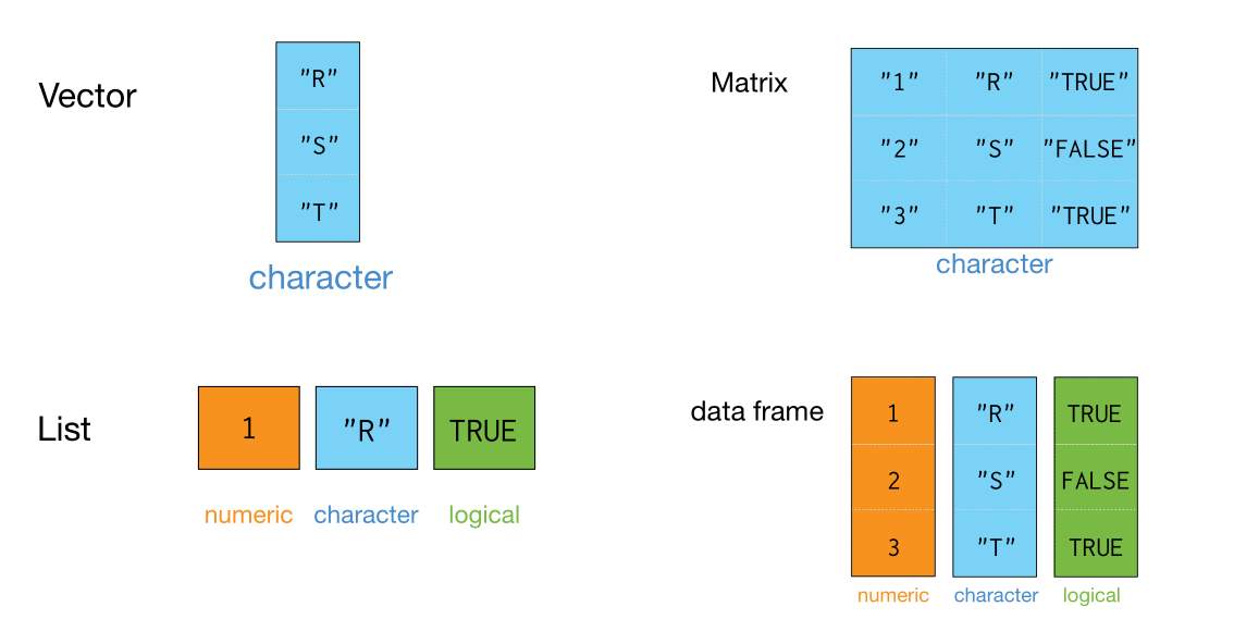
他们构造起来,很多相似性。
        list(a = 1, b = "a")   # list
           c(a = 1, b = 2)     # named vector
  data.frame(a = 1, b = 2)     # data frame
      tibble(a = 1, b = 2)     # tibble
- $a
- 1
- $b
- 'a'
- a
- 1
- b
- 2
| a | b |
|---|---|
| <dbl> | <dbl> |
| 1 | 2 |
| a | b |
|---|---|
| <dbl> | <dbl> |
| 1 | 2 |
向量化运算#
a <- c(2, 4, 3, 1, 5, 7)
用for()循环,让向量的每个元素乘以2
for (i in 1:length(a)){
    print(a[i] * 2)
}
[1] 4
[1] 8
[1] 6
[1] 2
[1] 10
[1] 14
事实上,R语言是支持向量化(将运算符或者函数作用在向量的每一个元素上),可以用向量化代替循环
a * 2
- 4
- 8
- 6
- 2
- 10
- 14
再比如,找出向量a中元素大于2的所有值
for (i in 1:length(a)){
    if (a[i] > 2)
        {print(a[i])}
}
[1] 4
[1] 3
[1] 5
[1] 7
用向量化的运算,可以轻松实现
a[a > 2]
- 4
- 3
- 5
- 7
列表#
a_list <- list(
  num = c(8,9),
  log = TRUE,
  cha = c("a", "b", "c")
)
a_list
- $num
-
- 8
- 9
- $log
- TRUE
- $cha
-
- 'a'
- 'b'
- 'c'
要想访问某个元素,可以这样
a_list["log"]
注意返回结果,第一行是$log,说明返回的结果仍然是列表, 相比a_list来说,a_list["log"]是只包含一个元素的列表。
将log元素里面的向量提取出来,就得用两个[[或者$
a_list[["log"]]
a_list$log
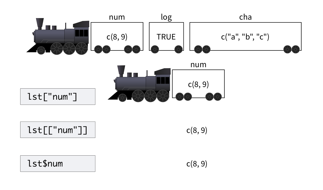
在tidyverse里,还可以用
a_list %>% pluck(1)
a_list %>% pluck("num")
- 8
- 9
- 8
- 9
列表 vs 向量#
v <- c(-2, -1, 0, 1, 2)
abs(v)
- 2
- 1
- 0
- 1
- 2
如果是列表形式,abs函数应用到列表中就会报错
lst <- list(-2, -1, 0, 1, 2)
abs(lst)
Error in abs(lst): 数学函数中用了非数值参数
Traceback:
用在向量的函数用在list上,往往行不通。
exams <- list(
  student1 = round(runif(10, 50, 100)),
  student2 = round(runif(10, 50, 100)),
  student3 = round(runif(10, 50, 100)),
  student4 = round(runif(10, 50, 100)),
  student5 = round(runif(10, 50, 100))
)
exams
- $student1
-
- 89
- 70
- 68
- 98
- 74
- 81
- 99
- 88
- 62
- 67
- $student2
-
- 75
- 57
- 76
- 94
- 73
- 76
- 73
- 72
- 84
- 66
- $student3
-
- 54
- 65
- 82
- 85
- 96
- 87
- 86
- 77
- 98
- 57
- $student4
-
- 65
- 70
- 71
- 90
- 81
- 86
- 55
- 90
- 76
- 86
- $student5
-
- 57
- 55
- 100
- 65
- 72
- 81
- 74
- 62
- 62
- 51
对列表执行向量函数的运算会很不方便
list(
  student1 = mean(exams$student1),
  student2 = mean(exams$student2),
  student3 = mean(exams$student3),
  student4 = mean(exams$student4),
  student5 = mean(exams$student5)
)
- $student1
- 79.6
- $student2
- 74.6
- $student3
- 78.7
- $student4
- 77
- $student5
- 67.9
purrr包#
对列表执行向量函数的运算
purrr::map(exams, mean)
- $student1
- 79.6
- $student2
- 74.6
- $student3
- 78.7
- $student4
- 77
- $student5
- 67.9
1 map函数#
map()函数的第一个参数是list或者vector, 第二个参数是函数
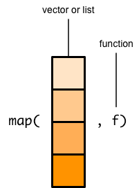
函数f应用到list/vector的每个元素
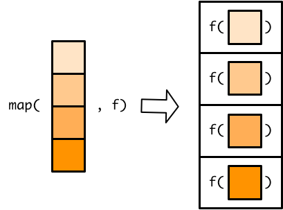
于是输入的 list/vector 中的每个元素,都对应一个输出
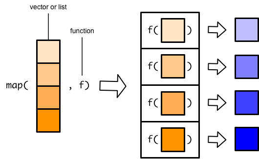
最后,所有的输出元素,聚合成一个新的list

在我们这个例子,mean() 作用到每个学生的成绩向量,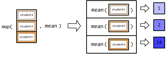 调用一次
调用一次mean(), 返回一个数值,所以最终的结果是五个数值的列表。
# 也可用管道
exams %>% map(mean)
- $student1
- 79.6
- $student2
- 74.6
- $student3
- 78.7
- $student4
- 77
- $student5
- 67.9
2 map函数家族#
map_dbl()返回的是数值型的向量map_dbl()要求每个输出的元素必须是数值型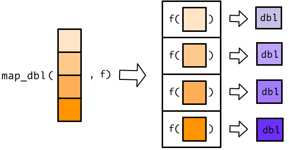
如果每个元素是数值型,
map_dbl()会聚合所有元素构成一个原子型向量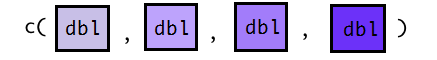
map_df()返回的结果是数据框
exams %>% map_dbl(mean)
- student1
- 79.6
- student2
- 74.6
- student3
- 78.7
- student4
- 77
- student5
- 67.9
exams %>% map_df(mean)
| student1 | student2 | student3 | student4 | student5 |
|---|---|---|---|---|
| <dbl> | <dbl> | <dbl> | <dbl> | <dbl> |
| 79.6 | 74.6 | 78.7 | 77 | 67.9 |
exams %>%
  data.frame() %>%
  map_df(mean)
| student1 | student2 | student3 | student4 | student5 |
|---|---|---|---|---|
| <dbl> | <dbl> | <dbl> | <dbl> | <dbl> |
| 79.6 | 74.6 | 78.7 | 77 | 67.9 |
3 map函数小结#
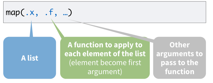
map函数第一个参数是向量或列表(数据框是列表的一种特殊形式,因此数据框也是可以的)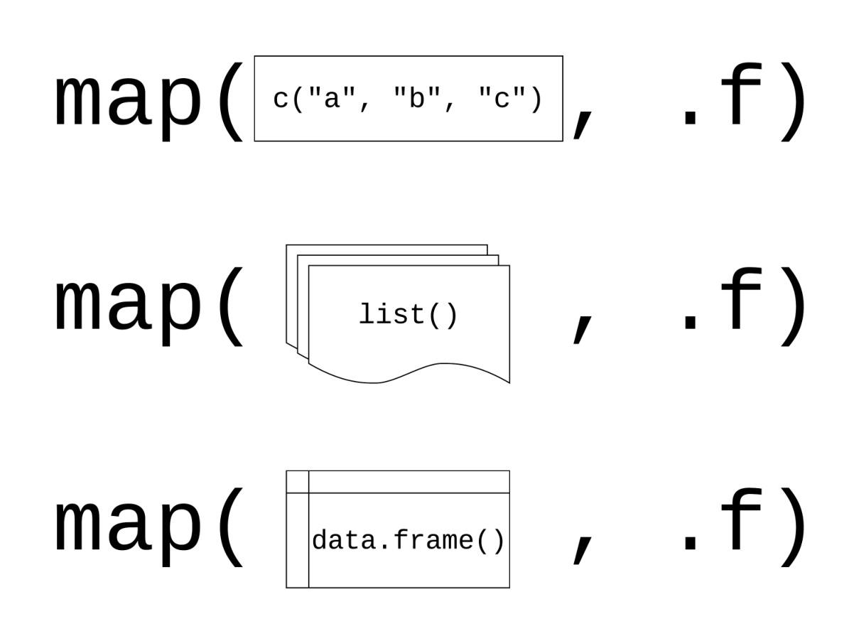
第二个参数是函数,这个函数会应用到列表的每一个元素,比如这里
map函数执行过程如下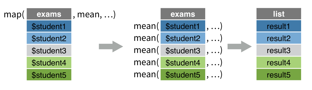
我们也可以根据需要,让map返回我们需要的数据格式, purrr也提供了方便的函数,具体如下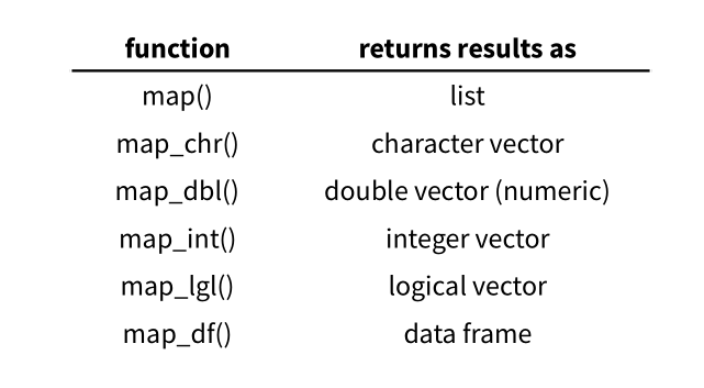
exams %>% map_df(var) # 方差
| student1 | student2 | student3 | student4 | student5 |
|---|---|---|---|---|
| <dbl> | <dbl> | <dbl> | <dbl> | <dbl> |
| 178.0444 | 96.04444 | 235.1222 | 136.6667 | 211.6556 |
4 额外参数#
在
sort()函数里添加参数decreasing = TRUE改为降序map很人性化,可以让函数的参数直接跟随在函数名之后,map()会自动的传递给函数。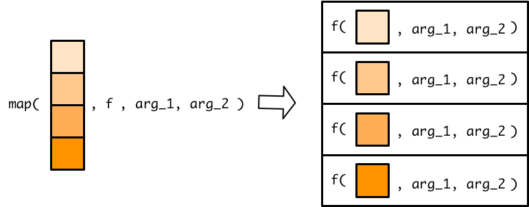
map(exams, sort) # 默认升序
map(exams, sort, decreasing=TRUE) # 改为降序
- $student1
-
- 62
- 67
- 68
- 70
- 74
- 81
- 88
- 89
- 98
- 99
- $student2
-
- 57
- 66
- 72
- 73
- 73
- 75
- 76
- 76
- 84
- 94
- $student3
-
- 54
- 57
- 65
- 77
- 82
- 85
- 86
- 87
- 96
- 98
- $student4
-
- 55
- 65
- 70
- 71
- 76
- 81
- 86
- 86
- 90
- 90
- $student5
-
- 51
- 55
- 57
- 62
- 62
- 65
- 72
- 74
- 81
- 100
- $student1
-
- 99
- 98
- 89
- 88
- 81
- 74
- 70
- 68
- 67
- 62
- $student2
-
- 94
- 84
- 76
- 76
- 75
- 73
- 73
- 72
- 66
- 57
- $student3
-
- 98
- 96
- 87
- 86
- 85
- 82
- 77
- 65
- 57
- 54
- $student4
-
- 90
- 90
- 86
- 86
- 81
- 76
- 71
- 70
- 65
- 55
- $student5
-
- 100
- 81
- 74
- 72
- 65
- 62
- 62
- 57
- 55
- 51
5 匿名函数#
我们也可以自定义函数。 比如我们这里定义了将向量中心化的函数(先求出10次考试的平均值,然后每次考试成绩去减这个平均值)
my_fun <- function(x){
    x - mean(x)
}
exams %>% map_df(my_fun)
| student1 | student2 | student3 | student4 | student5 |
|---|---|---|---|---|
| <dbl> | <dbl> | <dbl> | <dbl> | <dbl> |
| 9.4 | 0.4 | -24.7 | -12 | -10.9 |
| -9.6 | -17.6 | -13.7 | -7 | -12.9 |
| -11.6 | 1.4 | 3.3 | -6 | 32.1 |
| 18.4 | 19.4 | 6.3 | 13 | -2.9 |
| -5.6 | -1.6 | 17.3 | 4 | 4.1 |
| 1.4 | 1.4 | 8.3 | 9 | 13.1 |
| 19.4 | -1.6 | 7.3 | -22 | 6.1 |
| 8.4 | -2.6 | -1.7 | 13 | -5.9 |
| -17.6 | 9.4 | 19.3 | -1 | -5.9 |
| -12.6 | -8.6 | -21.7 | 9 | -16.9 |
我们也可以不用命名函数,而使用匿名函数。匿名函数顾名思义,就是没有名字的函数,
匿名函数直接放在map()函数中
exams %>%
  map_df(function(x){x - mean(x)})
| student1 | student2 | student3 | student4 | student5 |
|---|---|---|---|---|
| <dbl> | <dbl> | <dbl> | <dbl> | <dbl> |
| 9.4 | 0.4 | -24.7 | -12 | -10.9 |
| -9.6 | -17.6 | -13.7 | -7 | -12.9 |
| -11.6 | 1.4 | 3.3 | -6 | 32.1 |
| 18.4 | 19.4 | 6.3 | 13 | -2.9 |
| -5.6 | -1.6 | 17.3 | 4 | 4.1 |
| 1.4 | 1.4 | 8.3 | 9 | 13.1 |
| 19.4 | -1.6 | 7.3 | -22 | 6.1 |
| 8.4 | -2.6 | -1.7 | 13 | -5.9 |
| -17.6 | 9.4 | 19.3 | -1 | -5.9 |
| -12.6 | -8.6 | -21.7 | 9 | -16.9 |
还可以更加偷懒,用~代替function(),但代价是参数必须是规定的写法,比如.x
exams %>% map_df(~.x - mean(.x))
| student1 | student2 | student3 | student4 | student5 |
|---|---|---|---|---|
| <dbl> | <dbl> | <dbl> | <dbl> | <dbl> |
| 9.4 | 0.4 | -24.7 | -12 | -10.9 |
| -9.6 | -17.6 | -13.7 | -7 | -12.9 |
| -11.6 | 1.4 | 3.3 | -6 | 32.1 |
| 18.4 | 19.4 | 6.3 | 13 | -2.9 |
| -5.6 | -1.6 | 17.3 | 4 | 4.1 |
| 1.4 | 1.4 | 8.3 | 9 | 13.1 |
| 19.4 | -1.6 | 7.3 | -22 | 6.1 |
| 8.4 | -2.6 | -1.7 | 13 | -5.9 |
| -17.6 | 9.4 | 19.3 | -1 | -5.9 |
| -12.6 | -8.6 | -21.7 | 9 | -16.9 |
有时候,程序员觉得x还是有点多余,于是更够懒一点,只用., 也是可以的
exams %>% map_df(~. - mean(.))
| student1 | student2 | student3 | student4 | student5 |
|---|---|---|---|---|
| <dbl> | <dbl> | <dbl> | <dbl> | <dbl> |
| 9.4 | 0.4 | -24.7 | -12 | -10.9 |
| -9.6 | -17.6 | -13.7 | -7 | -12.9 |
| -11.6 | 1.4 | 3.3 | -6 | 32.1 |
| 18.4 | 19.4 | 6.3 | 13 | -2.9 |
| -5.6 | -1.6 | 17.3 | 4 | 4.1 |
| 1.4 | 1.4 | 8.3 | 9 | 13.1 |
| 19.4 | -1.6 | 7.3 | -22 | 6.1 |
| 8.4 | -2.6 | -1.7 | 13 | -5.9 |
| -17.6 | 9.4 | 19.3 | -1 | -5.9 |
| -12.6 | -8.6 | -21.7 | 9 | -16.9 |
~ 告诉 map() 后面跟随的是一个匿名函数,. 对应函数的参数,可以认为是一个占位符,等待传送带的student1、student2到student5 依次传递到函数机器。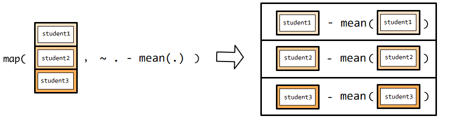
如果熟悉匿名函数的写法,会增强代码的可读性
exams %>%
  map_df(~length(.[. > 80]))
| student1 | student2 | student3 | student4 | student5 |
|---|---|---|---|---|
| <int> | <int> | <int> | <int> | <int> |
| 5 | 2 | 6 | 5 | 2 |
总之,有三种方法将函数传递给map()
直接传递
map(.x, mean, na.rm=TRUE)
Error in vctrs_vec_compat(.x, .purrr_user_env): 找不到对象'.x'
Traceback:

1. map(.x, mean, na.rm = TRUE)
2. map_("list", .x, .f, ..., .progress = .progress)
3. vctrs_vec_compat(.x, .purrr_user_env)
匿名函数
map(.x, funcition(.x){mean(.x, na.rm=TRUE)})
Error in parse(text = x, srcfile = src): <text>:1:22: 意外的'{'
1: map(.x, funcition(.x){
                         ^
Traceback:
使用
~
function(.x){.x*2}

~.x*2

map(.x, ~mean(.x, na.rm=TRUE))
function (.x)
{
    .x * 2
}
~.x * 2
Error in vctrs_vec_compat(.x, .purrr_user_env): 找不到对象'.x'
Traceback:

1. map(.x, ~mean(.x, na.rm = TRUE))
2. map_("list", .x, .f, ..., .progress = .progress)
3. vctrs_vec_compat(.x, .purrr_user_env)
在dplyr函数中的运用map#
1 在Tibble中#
Tibble本质上是向量构成的列表,因此tibble也适用map。假定有tibble如下
tb <-
  tibble(
    col_1 = c(1, 2, 3),
    col_2 = c(100, 200, 300),
    col_3 = c(0.1, 0.2, 0.3)
  )
map()中的函数f,可以作用到每一列
map_df(tb, median)
| col_1 | col_2 | col_3 |
|---|---|---|
| <dbl> | <dbl> | <dbl> |
| 2 | 200 | 0.2 |
在比如,找出企鹅数据中每列缺失值NA的数量
palmerpenguins::penguins %>%
  map_df(~sum(is.na(.)))
| species | island | bill_length_mm | bill_depth_mm | flipper_length_mm | body_mass_g | sex | year |
|---|---|---|---|---|---|---|---|
| <int> | <int> | <int> | <int> | <int> | <int> | <int> | <int> |
| 0 | 0 | 2 | 2 | 2 | 2 | 11 | 0 |
2 在col-column中#
如果想显示列表中每个元素的长度,可以这样写
tibble(
  x = list(1, 2:3, 4:6)
) %>%
  mutate(length = purrr::map_int(x, length))
| x | length |
|---|---|
| <list> | <int> |
| 1 | 1 |
| 2, 3 | 2 |
| 4, 5, 6 | 3 |
用于各种函数,比如产生随机数
tibble(
  x = c(3, 5, 6)
) %>%
  mutate(r = purrr::map(x, ~rnorm(., mean= 0, sd = 1)))
| x | r |
|---|---|
| <dbl> | <list> |
| 3 | -0.7442620, 0.2733458, 0.1971244 |
| 5 | -1.6398005, -0.1076375, 0.2406252, 0.1272739, 1.0788640 |
| 6 | -1.67253048, -0.69551409, -0.57144249, 1.36591820, 0.07352168, -1.36195263 |
用于建模
mtcars %>%
  group_by(cyl) %>%
  nest() %>%
  mutate(model = purrr::map(data, ~ lm(mpg ~ wt, data = .))) %>%
  mutate(result = purrr::map(model, ~ broom::tidy(.))) %>%
  unnest(result)
| cyl | data | model | term | estimate | std.error | statistic | p.value |
|---|---|---|---|---|---|---|---|
| <dbl> | <list> | <list> | <chr> | <dbl> | <dbl> | <dbl> | <dbl> |
| 6 | 21.000, 21.000, 21.400, 18.100, 19.200, 17.800, 19.700, 160.000, 160.000, 258.000, 225.000, 167.600, 167.600, 145.000, 110.000, 110.000, 110.000, 105.000, 123.000, 123.000, 175.000, 3.900, 3.900, 3.080, 2.760, 3.920, 3.920, 3.620, 2.620, 2.875, 3.215, 3.460, 3.440, 3.440, 2.770, 16.460, 17.020, 19.440, 20.220, 18.300, 18.900, 15.500, 0.000, 0.000, 1.000, 1.000, 1.000, 1.000, 0.000, 1.000, 1.000, 0.000, 0.000, 0.000, 0.000, 1.000, 4.000, 4.000, 3.000, 3.000, 4.000, 4.000, 5.000, 4.000, 4.000, 1.000, 1.000, 4.000, 4.000, 6.000 | 28.40884, -2.780106, -0.124967, 0.5839601, 1.929196, -0.689678, 0.3547199, -1.04528, -1.007951, -52.23469, -2.426656, 2.111436, -0.3526643, 0.679099, -0.720901, -1.10683, 2, 21.12497, 20.41604, 19.4708, 18.78968, 18.84528, 18.84528, 20.70795, 0, 1, -2.645751, 0.3779645, 0.3779645, 0.3779645, 0.3779645, 0.3779645, 0.3779645, -8.247185, 0.8728647, -0.2683341, -0.5490191, -0.526106, -0.526106, 0.2414814, 1.377964, 1.121188, 1, 2, 1e-07, 2, 5, lm(formula = mpg ~ wt, data = .), mpg ~ wt, 21, 21, 21.4, 18.1, 19.2, 17.8, 19.7, 2.62, 2.875, 3.215, 3.46, 3.44, 3.44, 2.77 | (Intercept) | 28.408845 | 4.1843688 | 6.789278 | 1.054844e-03 |
| 6 | 21.000, 21.000, 21.400, 18.100, 19.200, 17.800, 19.700, 160.000, 160.000, 258.000, 225.000, 167.600, 167.600, 145.000, 110.000, 110.000, 110.000, 105.000, 123.000, 123.000, 175.000, 3.900, 3.900, 3.080, 2.760, 3.920, 3.920, 3.620, 2.620, 2.875, 3.215, 3.460, 3.440, 3.440, 2.770, 16.460, 17.020, 19.440, 20.220, 18.300, 18.900, 15.500, 0.000, 0.000, 1.000, 1.000, 1.000, 1.000, 0.000, 1.000, 1.000, 0.000, 0.000, 0.000, 0.000, 1.000, 4.000, 4.000, 3.000, 3.000, 4.000, 4.000, 5.000, 4.000, 4.000, 1.000, 1.000, 4.000, 4.000, 6.000 | 28.40884, -2.780106, -0.124967, 0.5839601, 1.929196, -0.689678, 0.3547199, -1.04528, -1.007951, -52.23469, -2.426656, 2.111436, -0.3526643, 0.679099, -0.720901, -1.10683, 2, 21.12497, 20.41604, 19.4708, 18.78968, 18.84528, 18.84528, 20.70795, 0, 1, -2.645751, 0.3779645, 0.3779645, 0.3779645, 0.3779645, 0.3779645, 0.3779645, -8.247185, 0.8728647, -0.2683341, -0.5490191, -0.526106, -0.526106, 0.2414814, 1.377964, 1.121188, 1, 2, 1e-07, 2, 5, lm(formula = mpg ~ wt, data = .), mpg ~ wt, 21, 21, 21.4, 18.1, 19.2, 17.8, 19.7, 2.62, 2.875, 3.215, 3.46, 3.44, 3.44, 2.77 | wt | -2.780106 | 1.3349173 | -2.082605 | 9.175766e-02 |
| 4 | 22.800, 24.400, 22.800, 32.400, 30.400, 33.900, 21.500, 27.300, 26.000, 30.400, 21.400, 108.000, 146.700, 140.800, 78.700, 75.700, 71.100, 120.100, 79.000, 120.300, 95.100, 121.000, 93.000, 62.000, 95.000, 66.000, 52.000, 65.000, 97.000, 66.000, 91.000, 113.000, 109.000, 3.850, 3.690, 3.920, 4.080, 4.930, 4.220, 3.700, 4.080, 4.430, 3.770, 4.110, 2.320, 3.190, 3.150, 2.200, 1.615, 1.835, 2.465, 1.935, 2.140, 1.513, 2.780, 18.610, 20.000, 22.900, 19.470, 18.520, 19.900, 20.010, 18.900, 16.700, 16.900, 18.600, 1.000, 1.000, 1.000, 1.000, 1.000, 1.000, 1.000, 1.000, 0.000, 1.000, 1.000, 1.000, 0.000, 0.000, 1.000, 1.000, 1.000, 0.000, 1.000, 1.000, 1.000, 1.000, 4.000, 4.000, 4.000, 4.000, 4.000, 4.000, 3.000, 4.000, 5.000, 5.000, 4.000, 1.000, 2.000, 2.000, 1.000, 2.000, 1.000, 1.000, 1.000, 2.000, 2.000, 2.000 | 39.5712, -5.647025, -3.670097, 2.842815, 1.016934, 5.25226, -0.05125022, 4.691095, -4.151279, -1.344202, -1.486562, -0.6272468, -2.472466, -88.43328, 10.17096, 0.6947654, 6.230721, 1.728126, 6.169273, -3.535624, -0.00293297, -0.4259551, 1.291776, -2.288073, 2, 26.4701, 21.55719, 21.78307, 27.14774, 30.45125, 29.2089, 25.65128, 28.6442, 27.48656, 31.02725, 23.87247, 0, 1, -3.316625, 0.3015113, 0.3015113, 0.3015113, 0.3015113, 0.3015113, 0.3015113, 0.3015113, 0.3015113, 0.3015113, 0.3015113, -7.5809, -1.801119, 0.4754451, -0.05200489, -0.376803, -0.2546567, 0.0951259, -0.1991357, -0.08531752, -0.4334345, 0.2700172, 1.301511, 1.497654, 1, 2, 1e-07, 2, 9, lm(formula = mpg ~ wt, data = .), mpg ~ wt, 22.8, 24.4, 22.8, 32.4, 30.4, 33.9, 21.5, 27.3, 26, 30.4, 21.4, 2.32, 3.19, 3.15, 2.2, 1.615, 1.835, 2.465, 1.935, 2.14, 1.513, 2.78 | (Intercept) | 39.571196 | 4.3465820 | 9.103980 | 7.771511e-06 |
| 4 | 22.800, 24.400, 22.800, 32.400, 30.400, 33.900, 21.500, 27.300, 26.000, 30.400, 21.400, 108.000, 146.700, 140.800, 78.700, 75.700, 71.100, 120.100, 79.000, 120.300, 95.100, 121.000, 93.000, 62.000, 95.000, 66.000, 52.000, 65.000, 97.000, 66.000, 91.000, 113.000, 109.000, 3.850, 3.690, 3.920, 4.080, 4.930, 4.220, 3.700, 4.080, 4.430, 3.770, 4.110, 2.320, 3.190, 3.150, 2.200, 1.615, 1.835, 2.465, 1.935, 2.140, 1.513, 2.780, 18.610, 20.000, 22.900, 19.470, 18.520, 19.900, 20.010, 18.900, 16.700, 16.900, 18.600, 1.000, 1.000, 1.000, 1.000, 1.000, 1.000, 1.000, 1.000, 0.000, 1.000, 1.000, 1.000, 0.000, 0.000, 1.000, 1.000, 1.000, 0.000, 1.000, 1.000, 1.000, 1.000, 4.000, 4.000, 4.000, 4.000, 4.000, 4.000, 3.000, 4.000, 5.000, 5.000, 4.000, 1.000, 2.000, 2.000, 1.000, 2.000, 1.000, 1.000, 1.000, 2.000, 2.000, 2.000 | 39.5712, -5.647025, -3.670097, 2.842815, 1.016934, 5.25226, -0.05125022, 4.691095, -4.151279, -1.344202, -1.486562, -0.6272468, -2.472466, -88.43328, 10.17096, 0.6947654, 6.230721, 1.728126, 6.169273, -3.535624, -0.00293297, -0.4259551, 1.291776, -2.288073, 2, 26.4701, 21.55719, 21.78307, 27.14774, 30.45125, 29.2089, 25.65128, 28.6442, 27.48656, 31.02725, 23.87247, 0, 1, -3.316625, 0.3015113, 0.3015113, 0.3015113, 0.3015113, 0.3015113, 0.3015113, 0.3015113, 0.3015113, 0.3015113, 0.3015113, -7.5809, -1.801119, 0.4754451, -0.05200489, -0.376803, -0.2546567, 0.0951259, -0.1991357, -0.08531752, -0.4334345, 0.2700172, 1.301511, 1.497654, 1, 2, 1e-07, 2, 9, lm(formula = mpg ~ wt, data = .), mpg ~ wt, 22.8, 24.4, 22.8, 32.4, 30.4, 33.9, 21.5, 27.3, 26, 30.4, 21.4, 2.32, 3.19, 3.15, 2.2, 1.615, 1.835, 2.465, 1.935, 2.14, 1.513, 2.78 | wt | -5.647025 | 1.8501185 | -3.052251 | 1.374278e-02 |
| 8 | 18.700, 14.300, 16.400, 17.300, 15.200, 10.400, 10.400, 14.700, 15.500, 15.200, 13.300, 19.200, 15.800, 15.000, 360.000, 360.000, 275.800, 275.800, 275.800, 472.000, 460.000, 440.000, 318.000, 304.000, 350.000, 400.000, 351.000, 301.000, 175.000, 245.000, 180.000, 180.000, 180.000, 205.000, 215.000, 230.000, 150.000, 150.000, 245.000, 175.000, 264.000, 335.000, 3.150, 3.210, 3.070, 3.070, 3.070, 2.930, 3.000, 3.230, 2.760, 3.150, 3.730, 3.080, 4.220, 3.540, 3.440, 3.570, 4.070, 3.730, 3.780, 5.250, 5.424, 5.345, 3.520, 3.435, 3.840, 3.845, 3.170, 3.570, 17.020, 15.840, 17.400, 17.600, 18.000, 17.980, 17.820, 17.420, 16.870, 17.300, 15.410, 17.050, 14.500, 14.600, 0.000, 0.000, 0.000, 0.000, 0.000, 0.000, 0.000, 0.000, 0.000, 0.000, 0.000, 0.000, 0.000, 0.000, 0.000, 0.000, 0.000, 0.000, 0.000, 0.000, 0.000, 0.000, 0.000, 0.000, 0.000, 0.000, 1.000, 1.000, 3.000, 3.000, 3.000, 3.000, 3.000, 3.000, 3.000, 3.000, 3.000, 3.000, 3.000, 3.000, 5.000, 5.000, 2.000, 4.000, 3.000, 3.000, 3.000, 4.000, 4.000, 4.000, 2.000, 2.000, 4.000, 2.000, 4.000, 8.000 | 23.86803, -2.192438, 2.373957, -1.741026, 1.455193, 1.609764, -0.3806137, -1.95773, -1.576246, 2.550552, -0.6506476, -1.137005, -2.149067, 3.761895, -1.118001, -1.041026, -56.49903, -6.003055, 0.8157971, 1.220314, -0.8068206, -3.464586, -3.211015, 0.9738578, -0.8857193, -1.30959, -2.619382, 3.287904, -1.095775, -1.312854, 2, 16.32604, 16.04103, 14.94481, 15.69024, 15.58061, 12.35773, 11.97625, 12.14945, 16.15065, 16.337, 15.44907, 15.43811, 16.918, 16.04103, 0, 1, -3.741657, 0.2672612, 0.2672612, 0.2672612, 0.2672612, 0.2672612, 0.2672612, 0.2672612, 0.2672612, 0.2672612, 0.2672612, 0.2672612, 0.2672612, 0.2672612, -14.96369, 2.738073, -0.06892519, 0.05524975, 0.03698873, -0.4998852, -0.5634336, -0.5345812, 0.131946, 0.1629898, 0.0150755, 0.0132494, 0.2597732, 0.113685, 1.267261, 1.113685, 1, 2, 1e-07, 2, 12, lm(formula = mpg ~ wt, data = .), mpg ~ wt, 18.7, 14.3, 16.4, 17.3, 15.2, 10.4, 10.4, 14.7, 15.5, 15.2, 13.3, 19.2, 15.8, 15, 3.44, 3.57, 4.07, 3.73, 3.78, 5.25, 5.424, 5.345, 3.52, 3.435, 3.84, 3.845, 3.17, 3.57 | (Intercept) | 23.868029 | 3.0054619 | 7.941551 | 4.052705e-06 |
| 8 | 18.700, 14.300, 16.400, 17.300, 15.200, 10.400, 10.400, 14.700, 15.500, 15.200, 13.300, 19.200, 15.800, 15.000, 360.000, 360.000, 275.800, 275.800, 275.800, 472.000, 460.000, 440.000, 318.000, 304.000, 350.000, 400.000, 351.000, 301.000, 175.000, 245.000, 180.000, 180.000, 180.000, 205.000, 215.000, 230.000, 150.000, 150.000, 245.000, 175.000, 264.000, 335.000, 3.150, 3.210, 3.070, 3.070, 3.070, 2.930, 3.000, 3.230, 2.760, 3.150, 3.730, 3.080, 4.220, 3.540, 3.440, 3.570, 4.070, 3.730, 3.780, 5.250, 5.424, 5.345, 3.520, 3.435, 3.840, 3.845, 3.170, 3.570, 17.020, 15.840, 17.400, 17.600, 18.000, 17.980, 17.820, 17.420, 16.870, 17.300, 15.410, 17.050, 14.500, 14.600, 0.000, 0.000, 0.000, 0.000, 0.000, 0.000, 0.000, 0.000, 0.000, 0.000, 0.000, 0.000, 0.000, 0.000, 0.000, 0.000, 0.000, 0.000, 0.000, 0.000, 0.000, 0.000, 0.000, 0.000, 0.000, 0.000, 1.000, 1.000, 3.000, 3.000, 3.000, 3.000, 3.000, 3.000, 3.000, 3.000, 3.000, 3.000, 3.000, 3.000, 5.000, 5.000, 2.000, 4.000, 3.000, 3.000, 3.000, 4.000, 4.000, 4.000, 2.000, 2.000, 4.000, 2.000, 4.000, 8.000 | 23.86803, -2.192438, 2.373957, -1.741026, 1.455193, 1.609764, -0.3806137, -1.95773, -1.576246, 2.550552, -0.6506476, -1.137005, -2.149067, 3.761895, -1.118001, -1.041026, -56.49903, -6.003055, 0.8157971, 1.220314, -0.8068206, -3.464586, -3.211015, 0.9738578, -0.8857193, -1.30959, -2.619382, 3.287904, -1.095775, -1.312854, 2, 16.32604, 16.04103, 14.94481, 15.69024, 15.58061, 12.35773, 11.97625, 12.14945, 16.15065, 16.337, 15.44907, 15.43811, 16.918, 16.04103, 0, 1, -3.741657, 0.2672612, 0.2672612, 0.2672612, 0.2672612, 0.2672612, 0.2672612, 0.2672612, 0.2672612, 0.2672612, 0.2672612, 0.2672612, 0.2672612, 0.2672612, -14.96369, 2.738073, -0.06892519, 0.05524975, 0.03698873, -0.4998852, -0.5634336, -0.5345812, 0.131946, 0.1629898, 0.0150755, 0.0132494, 0.2597732, 0.113685, 1.267261, 1.113685, 1, 2, 1e-07, 2, 12, lm(formula = mpg ~ wt, data = .), mpg ~ wt, 18.7, 14.3, 16.4, 17.3, 15.2, 10.4, 10.4, 14.7, 15.5, 15.2, 13.3, 19.2, 15.8, 15, 3.44, 3.57, 4.07, 3.73, 3.78, 5.25, 5.424, 5.345, 3.52, 3.435, 3.84, 3.845, 3.17, 3.57 | wt | -2.192438 | 0.7392393 | -2.965803 | 1.179281e-02 |
# midify会修改原始数据,推荐使用map
exams %>% map_df(~ . - mean(.))

exams %>% modify(~ . - mean(.))
| student1 | student2 | student3 | student4 | student5 |
|---|---|---|---|---|
| <dbl> | <dbl> | <dbl> | <dbl> | <dbl> |
| 9.4 | 0.4 | -24.7 | -12 | -10.9 |
| -9.6 | -17.6 | -13.7 | -7 | -12.9 |
| -11.6 | 1.4 | 3.3 | -6 | 32.1 |
| 18.4 | 19.4 | 6.3 | 13 | -2.9 |
| -5.6 | -1.6 | 17.3 | 4 | 4.1 |
| 1.4 | 1.4 | 8.3 | 9 | 13.1 |
| 19.4 | -1.6 | 7.3 | -22 | 6.1 |
| 8.4 | -2.6 | -1.7 | 13 | -5.9 |
| -17.6 | 9.4 | 19.3 | -1 | -5.9 |
| -12.6 | -8.6 | -21.7 | 9 | -16.9 |
- $student1
-
- 9.40000000000001
- -9.59999999999999
- -11.6
- 18.4
- -5.59999999999999
- 1.40000000000001
- 19.4
- 8.40000000000001
- -17.6
- -12.6
- $student2
-
- 0.400000000000006
- -17.6
- 1.40000000000001
- 19.4
- -1.59999999999999
- 1.40000000000001
- -1.59999999999999
- -2.59999999999999
- 9.40000000000001
- -8.59999999999999
- $student3
-
- -24.7
- -13.7
- 3.3
- 6.3
- 17.3
- 8.3
- 7.3
- -1.7
- 19.3
- -21.7
- $student4
-
- -12
- -7
- -6
- 13
- 4
- 9
- -22
- 13
- -1
- 9
- $student5
-
- -10.9
- -12.9
- 32.1
- -2.90000000000001
- 4.09999999999999
- 13.1
- 6.09999999999999
- -5.90000000000001
- -5.90000000000001
- -16.9
函数式编程2#
事实上,purrr()家族还有其它map()函数,可以在多个向量中迭代。也就说,同时接受多个向量的元素,并行计算。比如,map2()函数可以处理两个向量,而pmap()函数可以处理更多向量。
library(tidyverse)
map2()#
map2()函数和map()函数类似,不同在于map2()接受两个的向量,这两个向量必须是等长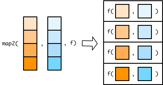 在
在map()函数使用匿名函数,可以用 . 代表输入向量的每个元素。在map2()函数, .不够用,所有需要需要用 .x 代表第一个向量的元素,.y代表第二个向量的元素
x <- c(1,2,3)
y <- c(4,5,6)

map2(x, y, ~.x + .y)
- 5
- 7
- 9
tibble的每一列都是向量,所以可以把map2()放在mutate()函数内部,对tibble的多列同时迭代
df <- tibble(
  a = c(1, 2, 3),
  b = c(4, 5, 6)
)

df %>%
  mutate(min = map2(a, b, ~min(.x, .y)))
| a | b | min |
|---|---|---|
| <dbl> | <dbl> | <list> |
| 1 | 4 | 1 |
| 2 | 5 | 2 |
| 3 | 6 | 3 |
也可以简写
df %>%
  mutate(min = map2_dbl(a, b, min))
| a | b | min |
|---|---|---|
| <dbl> | <dbl> | <dbl> |
| 1 | 4 | 1 |
| 2 | 5 | 2 |
| 3 | 6 | 3 |
mutate() 是column-operation,即提取数据框一列作为向量,传递到mutate中,map2_dbl()返回的也是一个等长的向量。
因此,也可以用rowwise()逐行应用函数
df %>%
  rowwise() %>%
  mutate(min = min(a, b)) %>%
  ungroup()
| a | b | min |
|---|---|---|
| <dbl> | <dbl> | <dbl> |
| 1 | 4 | 1 |
| 2 | 5 | 2 |
| 3 | 6 | 3 |
pmap()#
没有map3()或者map4()函数,只有 pmap() 函数可用(p 的意思是 parallel)
purrr::pmap()函数稍微有点不一样的地方:
map()和map2()函数,指定传递给函数f的向量,向量各自放在各自的位置上pmap()需要将传递给函数的向量名,先装入一个list()中, 再传递给函数f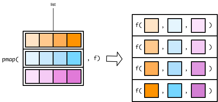 翻转列表的图示,参数的传递关系看地更清楚。
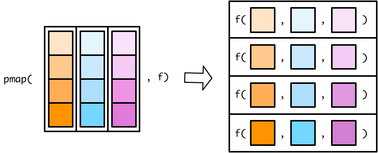
事实上,map2()是pmap()的一种特殊情况
map2_dbl(x, y, min)
- 1
- 2
- 3
pmap_dbl(list(x, y), min)
- 1
- 2
- 3
1 用在tibble#
tibble本质上就是list,这种结构就是pmap()所需要的,因此,直接应用函数即可。
tibble(
  a = c(50, 60, 70),
  b = c(10, 90, 40),
  c = c(1, 105, 200)
) %>%
  pmap_dbl(min)
- 1
- 60
- 40
2 匿名函数#
pmap()可以接受多个向量,因此在pmap()中使用匿名函数,就需要一种新的方法来标识每个向量。
由于向量是多个,因此不再用.x, .y,而是用..1, ..2, ..3 分别代表第一个向量、第二个向量和第三个向量。
pmap(
  list(1:5, 5:1, 2), ~..1 + ..2 + ..3
)
- 8
- 8
- 8
- 8
- 8
3 命名函数#
runif()产生均匀分布随机数
params <- tibble::tribble(
  ~ n, ~ min, ~ max,
   1L,     0,     1,
   2L,    10,   100,
   3L,   100,  1000
)
pmap(params, ~runif(n = ..1, min = ..2, max = ..3))
- 0.0769681525416672
-
- 28.0839628400281
- 41.5693232929334
-
- 199.041049205698
- 191.574636357836
- 512.634686636738
如果提供给pmap()的.f 是命名函数,比如runif(n, min = , max = ),它有三个参数 n, min, max, 而我们输入的列表刚好也有三个同名的元素,那么他们会自动匹配,代码因此变得更加简练
pmap(params, runif)
- 0.959976142272353
-
- 13.1245567044243
- 59.6250989451073
-
- 590.096804616041
- 511.394972563721
- 332.652951683849
当然,这里需要注意的是
输入列表的元素,其个数要与函数的参数个数一致
输入列表的元素,其变量名也要与函数的参数名一致
其他purrr函数#
1 Map functions that output tibbles#
接着介绍purrr宏包的其他函数。 map()家族除了返回list和atomic vector 外,map_df(), map_dfr() 和map_dfc()还可以返回tibble。
这个过程,好比生产线上的工人把输入的列表元素依次转换成一个个tibble,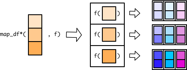 最后归集一个大的
tibble。在归集成一个大的tibble的时候,有两种方式,
竖着堆积,
map_dfr()(r for rows)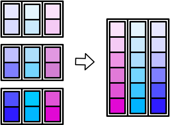
并排堆放
map_dfc()(c for columns)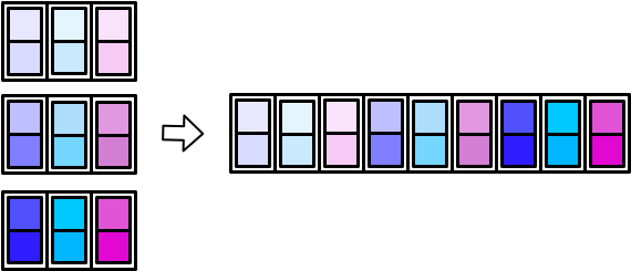
2 Walk and friends#
walk()函数与map()系列函数类似,但应用场景不同,map()在于执行函数操作,而walk() 保存记录数据(比如print(),write.csv(), ggsave()),常用于保存数据和生成图片。比如我们用map()生成系列图片,
plot_rnorm <- function(sd){
    tibble(x = rnorm(n = 5000, mean = 0, sd = sd)) %>%
      ggplot(aes(x)) +
      geom_histogram(bins = 40) +
      geom_vline(xintercept = 0, color = "blue")
}

plots <-
  c(5, 1, 9) %>%
  map(plot_rnorm)

plots %>%
  walk(print)
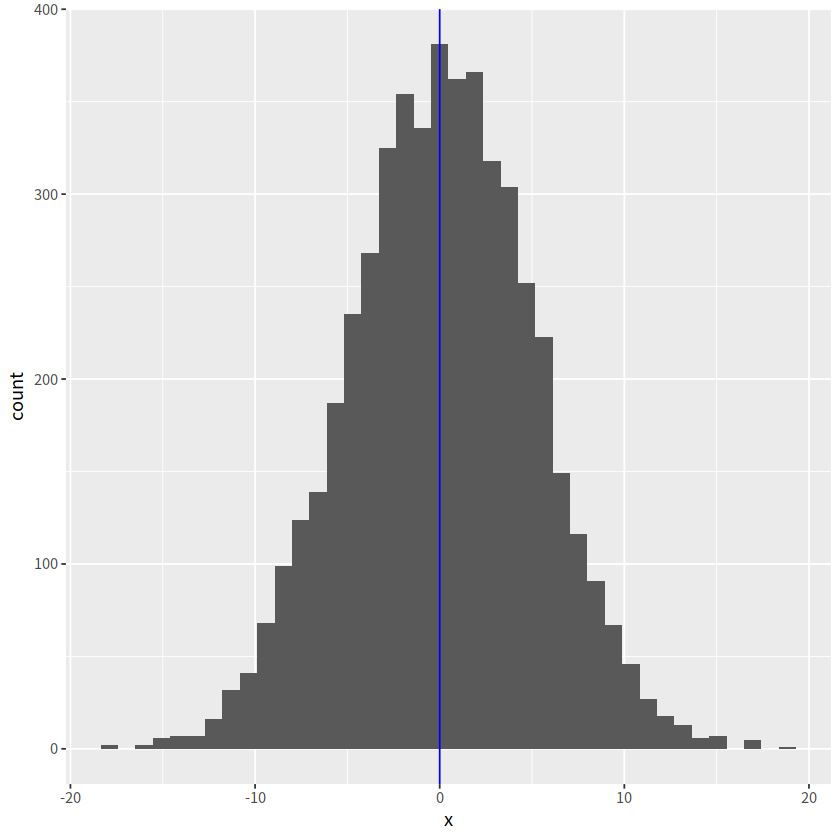
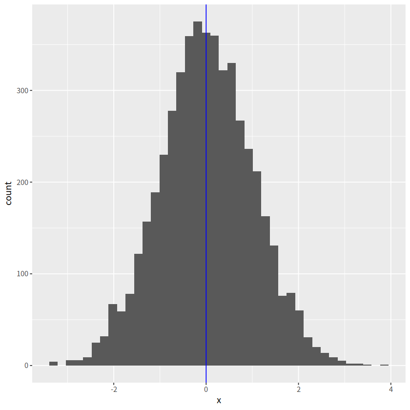
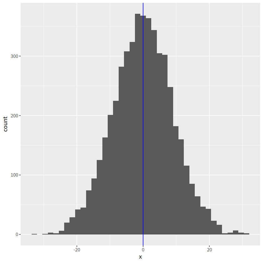
map()函数是一定要返回列表的,但walk()看上去函数没有返回值,实际上它返回的就是它的输入,只是用户不可见而已。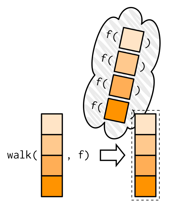 这样的设计很有用,尤其在管道操作中,我们可以统计中,用
walk()保存中间计算的结果或者生成图片,然后若无其事地继续管道(因为walk()返回值,就是输入walk的值),保持计算的连贯。