library(tidyverse) # install.packages("tidyverse")
library(patchwork) # install.packages("patchwork")

── Attaching core tidyverse packages ───────────────────────────────────────────────────────────────────────────────────────────────────────────────────────── tidyverse 2.0.0 ──
✔ dplyr     1.1.4     ✔ readr     2.1.5
✔ forcats   1.0.0     ✔ stringr   1.5.1
✔ ggplot2   3.5.0     ✔ tibble    3.2.1
✔ lubridate 1.9.3     ✔ tidyr     1.3.1
✔ purrr     1.0.2     

── Conflicts ─────────────────────────────────────────────────────────────────────────────────────────────────────────────────────────────────────────── tidyverse_conflicts() ──
✖ dplyr::filter() masks stats::filter()
✖ dplyr::lag()    masks stats::lag()
ℹ Use the conflicted package (<http://conflicted.r-lib.org/>) to force all conflicts to become errors

数据可视化-ggplot入门

图形属性

• 我们在图中画一个点，那么这个点就有（形状，大小，颜色，位置，透明度）等属性， 这些属性就是图形属性（有时也称之为图形元素或者视觉元素）

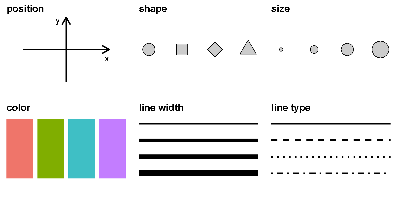
• 点和线常用的图形属性

geom	x	y	size	color	shape	linetype	alpha	fill	group
point	√	√	√	√	√	√	√	√	√
line	√	√	√	√		√	√		√

宏包ggplot2

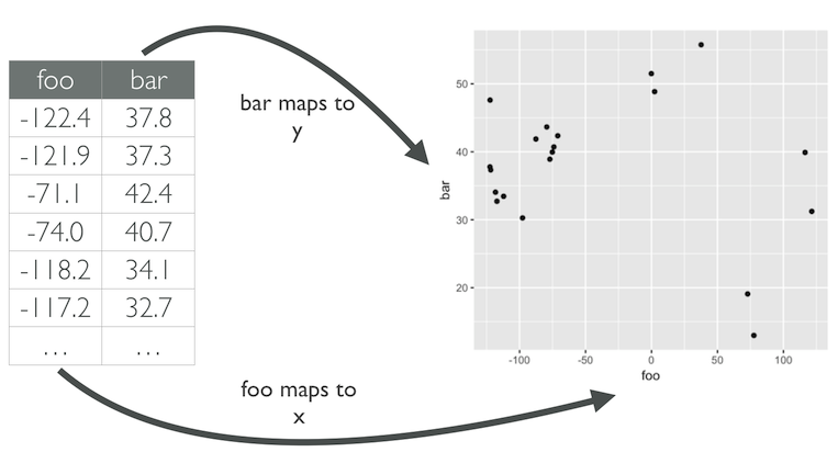
• ggplot2有一套优雅的绘图语法，包名中“gg”是grammar of graphics的简称。

• 数值到图形属性的映射过程

  • 

• 我们希望用点的大小代表这个位置上的某个变量（比如，降雨量，产品销量等等），那么变量的数值越小，点的半径就小一点，数值越大，点就可以大一点；或者变量的数值大，点的颜色就深一点，数值小，点的颜色就浅一点。即，数值到图形属性的映射过程。

• 映射是一个数学词汇，可以理解为一一对应。

1 ggplot()函数包括9个部件

• 数据 (data) （数据框）

• 映射 (mapping)

• 几何形状 (geom)

• 统计变换 (stats)

• 标度 (scale)

• 坐标系 (coord)

• 分面 (facet)

• 主题 (theme)

• 存储和输出 (output)

其中数据、映射、几何形状这三个是必需的。 语法模版如下

ggplot(data = <DATA>) + 
   <GEOM_FUNCTION>(mapping = aes(<MAPPINGS>))

Error in parse(text = x, srcfile = src): <text>:1:15: 意外的'<'
1: ggplot(data = <
                  ^
Traceback:

此外，图形中还可能包含数据的统计变换(statistical transformation，缩写stats)，最后绘制在某个特定的坐标系(coordinate system，缩写coord)中，而分面(facet)则可以用来生成数据不同子集的图形。

library(tidyverse)
library(janitor)
library(palmerpenguins)

penguins <- penguins %>% 
  janitor::clean_names() %>% 
  drop_na()

载入程辑包：‘janitor’

The following objects are masked from ‘package:stats’:

    chisq.test, fisher.test

penguins %>% 
  head()

A tibble: 6 × 8

species	island	bill_length_mm	bill_depth_mm	flipper_length_mm	body_mass_g	sex	year
<fct>	<fct>	<dbl>	<dbl>	<int>	<int>	<fct>	<int>
Adelie	Torgersen	39.1	18.7	181	3750	male	2007
Adelie	Torgersen	39.5	17.4	186	3800	female	2007
Adelie	Torgersen	40.3	18.0	195	3250	female	2007
Adelie	Torgersen	36.7	19.3	193	3450	female	2007
Adelie	Torgersen	39.3	20.6	190	3650	male	2007
Adelie	Torgersen	38.9	17.8	181	3625	female	2007

penguins %>% 
  select(species, sex, bill_length_mm, bill_depth_mm) %>% 
  head(4)

A tibble: 4 × 4

species	sex	bill_length_mm	bill_depth_mm
<fct>	<fct>	<dbl>	<dbl>
Adelie	male	39.1	18.7
Adelie	female	39.5	17.4
Adelie	female	40.3	18.0
Adelie	female	36.7	19.3

ggplot(data = penguins)+
  geom_point(aes(x = bill_length_mm, y = bill_depth_mm,
                 size=species, color=species,
                shape=species, alpha=sex))

Warning message:
“Using size for a discrete variable is not advised.”

Warning message:
“Using alpha for a discrete variable is not advised.”

• 

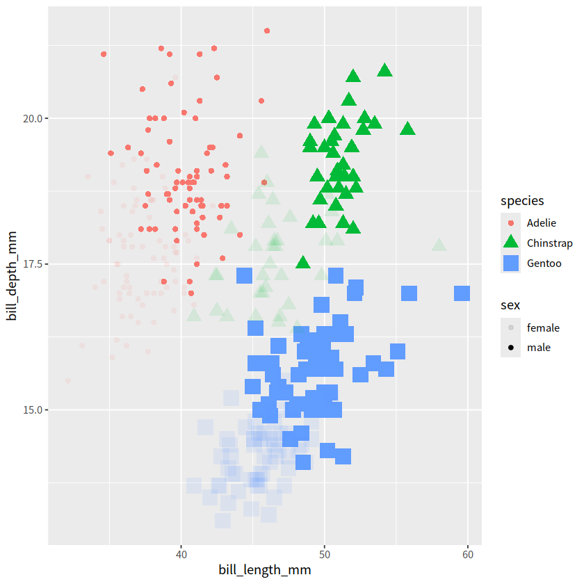
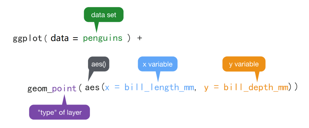
• ggplot() 初始化绘图，相当于打开了一张纸，准备画画。

• ggplot(data = penguins) 表示使用penguins这个数据框来画图。

• +表示添加图层。

• geom_point()表示绘制散点图。

• aes()表示数值和视觉属性之间的映射。

• aes()除了位置上映射，还可以实现**色彩(color)、形状(size)或透明度(alpha)**等视觉属性的映射。

aes(x = bill_length_mm, y = bill_depth_mm)，意思是变量bill_length_mm作为（映射为）x轴方向的位置，变量bill_depth_mm作为（映射为）y轴方向的位置。

• ggplot()内部有一套默认的设置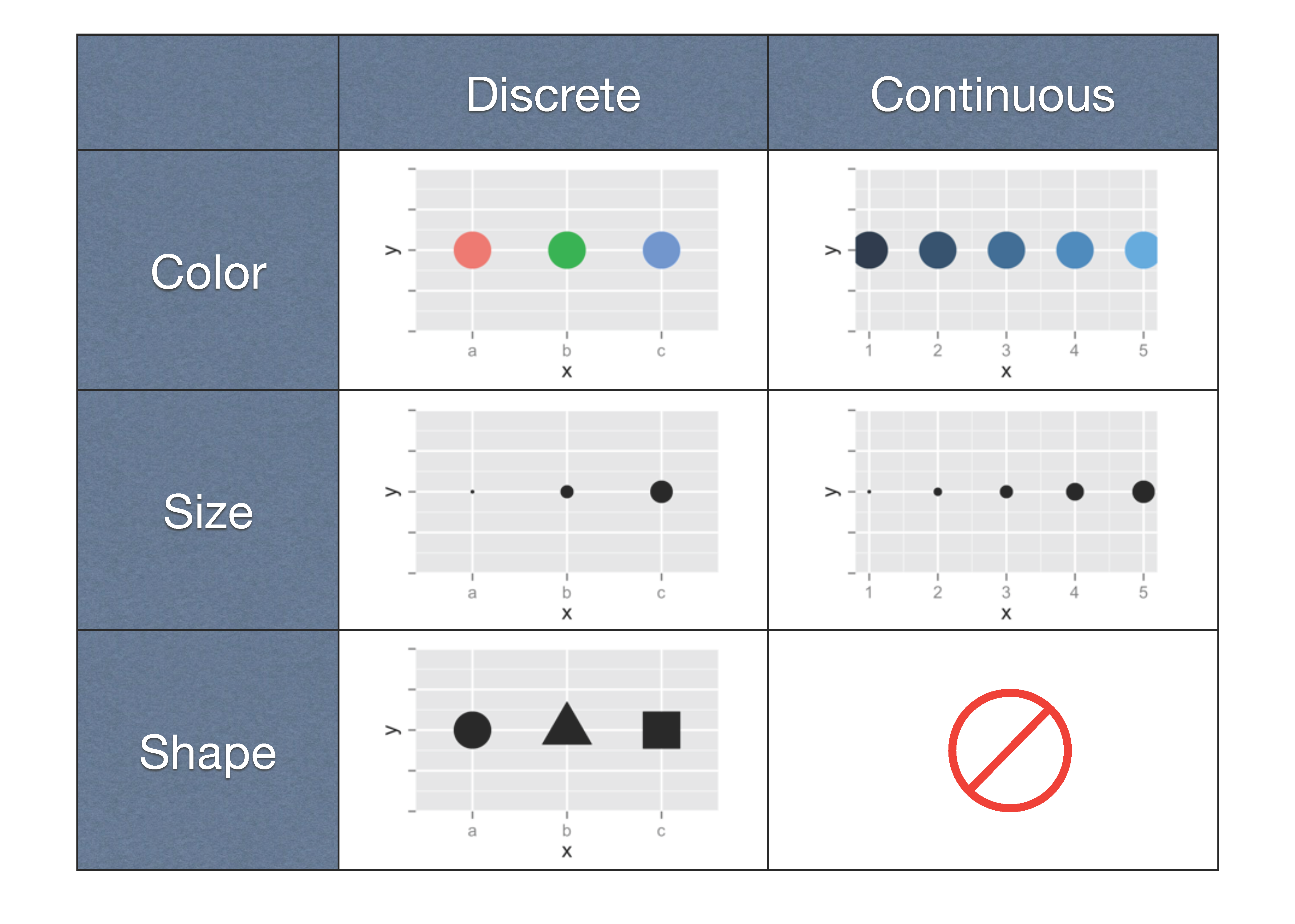

• 

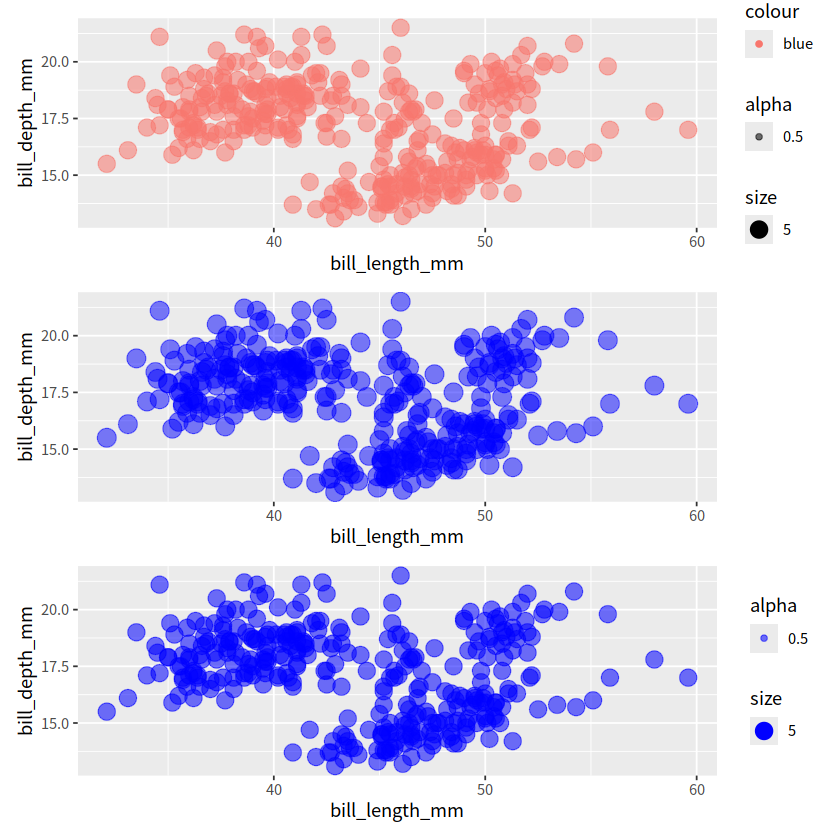
2 映射 vs 设置

• 想把图中的点指定为某一种颜色，可以使用设置语句，比如

## 映射只是将你提供的元素映射进图片中，
## 而设置则会按照想要的方式设置某些元素
p1 = ggplot(penguins)+
  geom_point(aes(x = bill_length_mm, y = bill_depth_mm,
                 color = "blue", size=5, alpha=0.5) 
             )

p2 = ggplot(penguins)+
  geom_point(aes(x = bill_length_mm, y = bill_depth_mm), 
             color = "blue", size=5, alpha=0.5)

p1 / p2 / ggplot(penguins)+
             geom_point(aes(x = bill_length_mm, y = bill_depth_mm,
                        color = "blue", size=5, alpha=0.5), 
                        color="blue")
## 所以p1中只是将"blue"这个元素映射入图片的color，表示只有一种类型的颜色
# 不会改变图片的颜色属性，这是我的个人理解

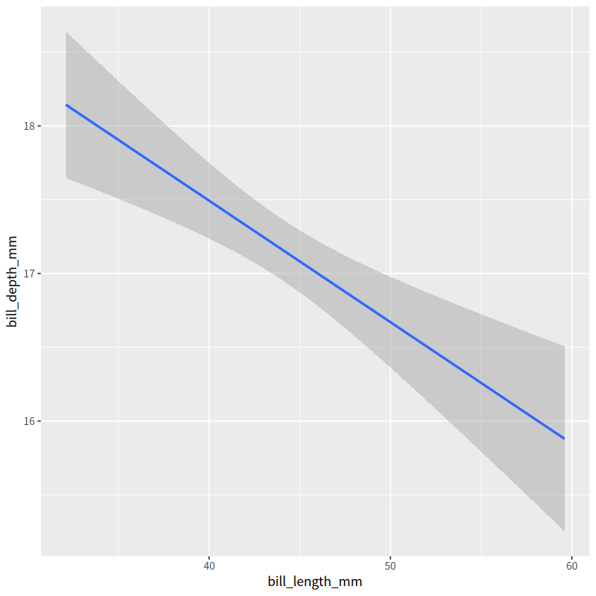
3 几何形状

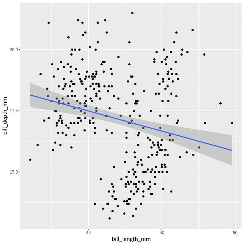
• geom_point() 可以画散点图，也可以使用geom_smooth()绘制平滑曲线

• geom_smooth()有多个绘制平滑曲线的方法——线性拟合

ggplot(penguins) +
  geom_smooth(aes(x = bill_length_mm, y = bill_depth_mm),
             method = "lm")

`geom_smooth()` using formula = 'y ~ x'

4 图层叠加

ggplot(penguins)+
  geom_point(aes(x = bill_length_mm, y = bill_depth_mm))+
  geom_smooth(aes(x = bill_length_mm, y = bill_depth_mm), method="lm")

`geom_smooth()` using formula = 'y ~ x'

## 如果两图层使用的x y 相同，则可以直接将元素映射到底层(公用)ggplot()中
ggplot(penguins, aes(x = bill_length_mm, y = bill_depth_mm))+
  geom_point()+
  geom_smooth(method="lm")

`geom_smooth()` using formula = 'y ~ x'

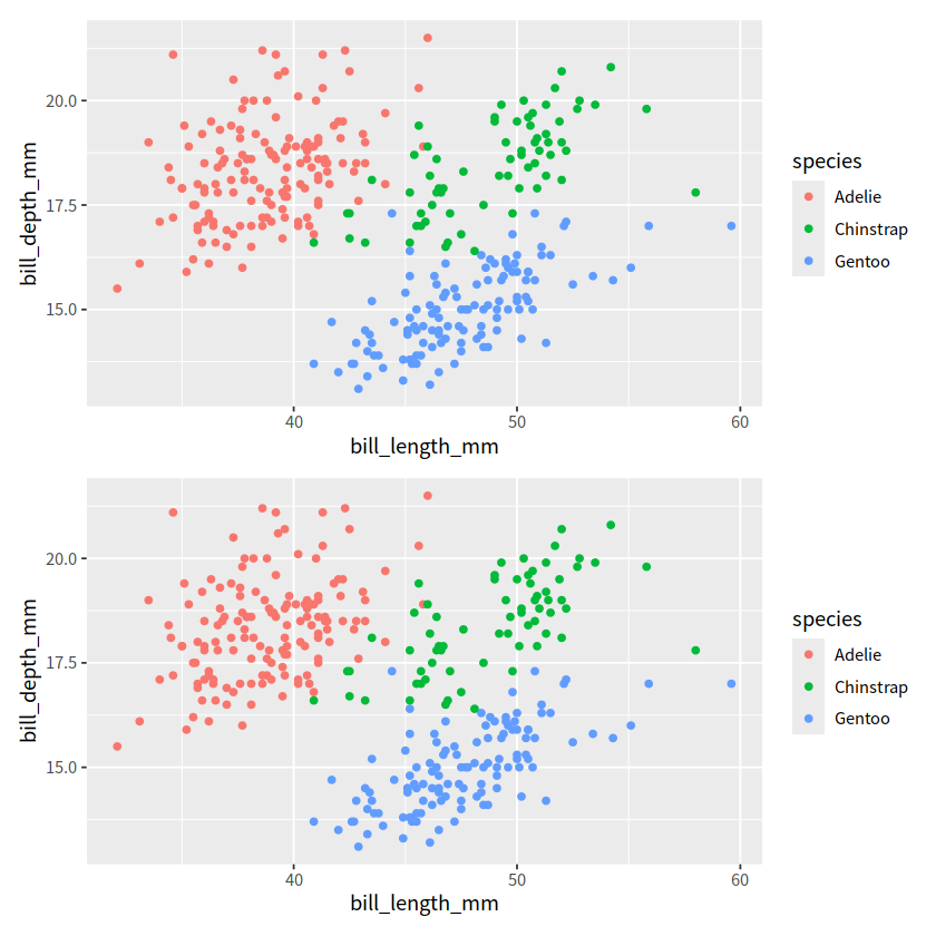
5 Global vs Local

• 以下两段代码出来的图是一样。但背后的含义却不同。

• 映射关系aes(x = bill_length_mm, y = bill_depth_mm) 写在ggplot()里, 为全局声明(Global)。

  • 那么，当geom_point()画图时，发现缺少图形所需要的映射关系（点的位置、点的大小、点的颜色等等），就会从ggplot()全局变量中继承映射关系。

• 如果映射关系aes(x = bill_length_mm, y = bill_depth_mm)写在几何形状geom_point()里, 那么此处的映射关系就为局部声明(Local)

  • 那么geom_point()绘图时，发现所需要的映射关系已经存在，就不会继承全局变量的映射关系。

p1 = ggplot(penguins, aes(x=bill_length_mm, y=bill_depth_mm, 
                          color=species))+
       geom_point()

p2 = ggplot(penguins) +
       geom_point(aes(x = bill_length_mm, y = bill_depth_mm, 
                      color = species))
p1/p2

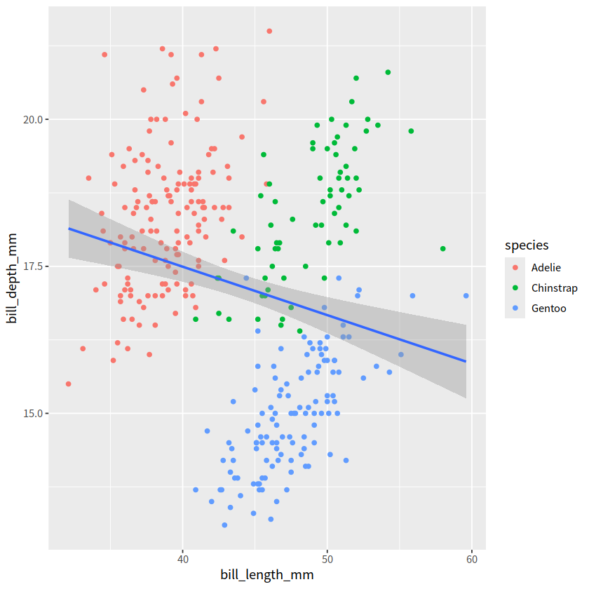
ggplot(penguins, aes(x = bill_length_mm, y = bill_depth_mm))+
  geom_point(aes(color=species))+
  geom_smooth(method="lm")
# 这里的 geom_point() 和 geom_smooth() 都会从全局变量中继承位置映射关系

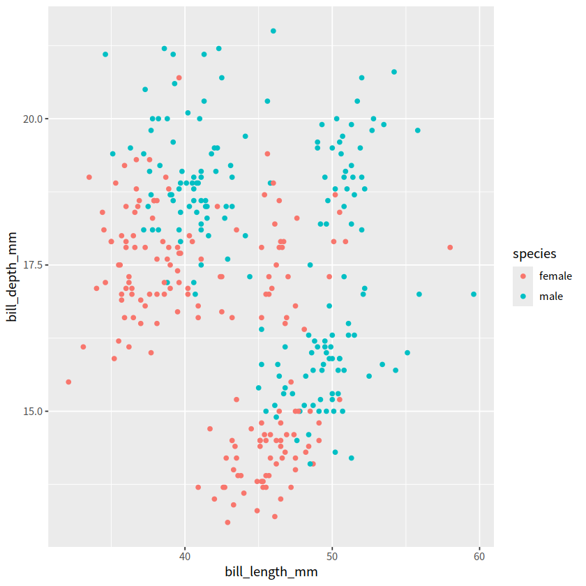
ggplot(penguins,aes(x = bill_length_mm, y = bill_depth_mm, color = species)) +
  geom_point(aes(color = sex))
# 局部变量中的映射关系aes(color=)已经存在，因此不会从全局变量中继承
# 沿用当前的映射关系

`geom_smooth()` using formula = 'y ~ x'

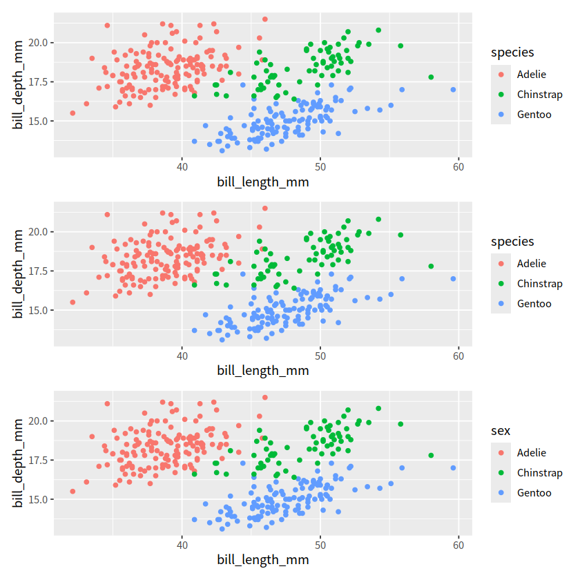
### 图层从全局声明中继承
# 当当前local单独声明时，图例标题还是会继承全局声明，而图例内容则沿用当前
p1 = ggplot(penguins, aes(x = bill_length_mm, y = bill_depth_mm, color = species)) +
      geom_point()

p2 = ggplot(penguins, aes(x = bill_length_mm, y = bill_depth_mm)) +
      geom_point(aes(color = species))

p3 = ggplot(penguins, aes(x = bill_length_mm, y = bill_depth_mm, color = sex)) +
      geom_point(aes(color = species))
# p3图例的标题继承了全局声明中的color
p1/p2/p3

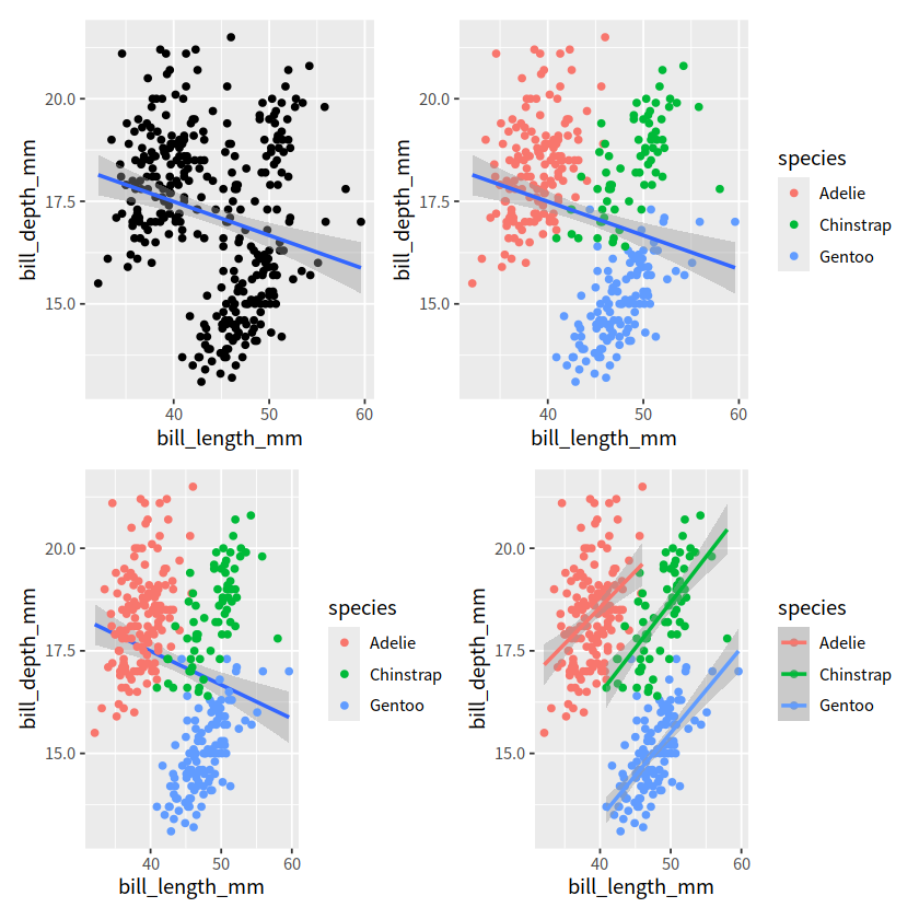
### 图层之间没有继承关系
p1 = ggplot(penguins, aes(x = bill_length_mm, y = bill_depth_mm)) +
       geom_point() +
       geom_smooth(method = "lm")


p2 = ggplot(penguins, aes(x = bill_length_mm, y = bill_depth_mm)) +
       geom_point(aes(color = species)) +
       geom_smooth(method = "lm")

p3 = ggplot(penguins, aes(x = bill_length_mm, y = bill_depth_mm)) +
       geom_smooth(method = "lm") +
       geom_point(aes(color = species))

p4 = ggplot(penguins, aes(x = bill_length_mm, y = bill_depth_mm, color = species)) +
       geom_point() +
       geom_smooth(method = "lm") 

(p1 + p2) / (p3 + p4)

`geom_smooth()` using formula = 'y ~ x'

`geom_smooth()` using formula = 'y ~ x'

`geom_smooth()` using formula = 'y ~ x'

`geom_smooth()` using formula = 'y ~ x'

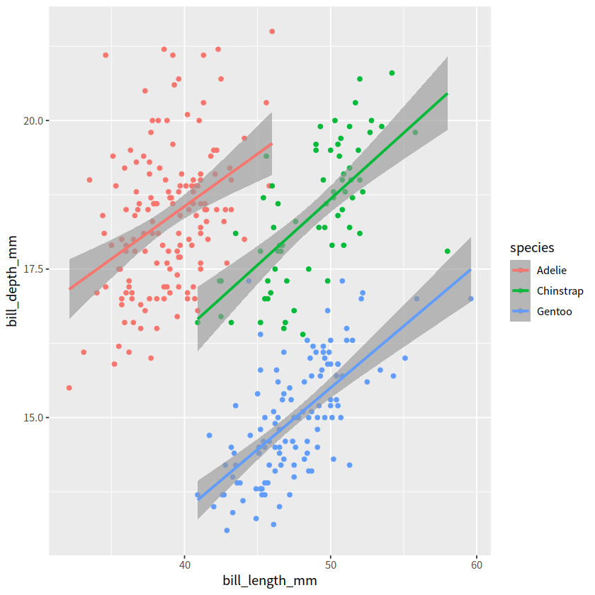
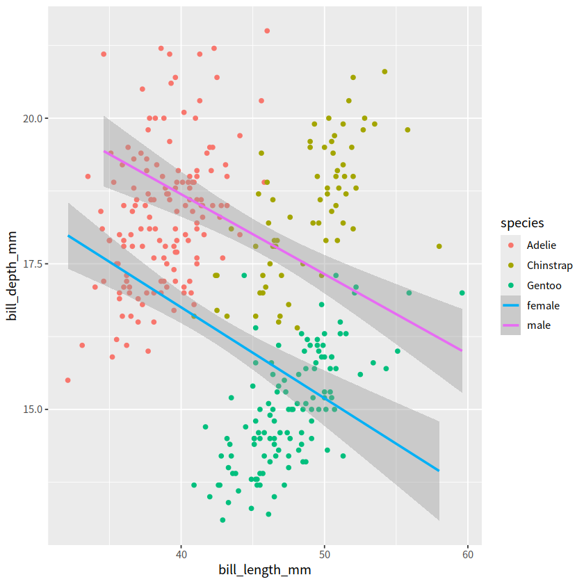
ggplot(penguins, aes(x = bill_length_mm, y = bill_depth_mm, color = species)) +
  geom_point() +
  geom_smooth(method = "lm", aes(color = sex)) 

`geom_smooth()` using formula = 'y ~ x'

6 保存图片

• ggsave()函数，将图片保存为所需要的格式，如”.pdf”, “.png”等， 还可以指定图片的高度和宽度，默认units是英寸，也可以使用”cm”, or “mm”.

• 如果想保存当前图形，ggplot()可以不用赋值，同时省略ggsave()中的 plot = p1，ggsave()会自动保存最近一次的绘图

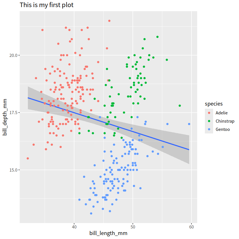
p1 <- penguins %>% 
  ggplot(aes(x = bill_length_mm, y = bill_depth_mm)) +
  geom_smooth(method = lm) +
  geom_point(aes(color = species)) +
  ggtitle("This is my first plot")
p1

ggsave(plot=p1, filename="my_plot.pdf", width=8, height=5, dpi=330)

`geom_smooth()` using formula = 'y ~ x'

`geom_smooth()` using formula = 'y ~ x'

penguins %>% 
  ggplot(aes(x = bill_length_mm, y = bill_depth_mm)) +
  geom_smooth(method = lm) +
  geom_point(aes(color = species)) +
  ggtitle("This is my first plot")

ggsave("my_last_plot.pdf", width = 8, height = 6, dpi = 330)

`geom_smooth()` using formula = 'y ~ x'

`geom_smooth()` using formula = 'y ~ x'

ggplot(penguins, aes(x = bill_length_mm, y = bill_depth_mm, color=species)) +
  geom_point() +
  geom_smooth(method="lm") +
  geom_smooth(aes(color=species), method="lm") 

`geom_smooth()` using formula = 'y ~ x'

`geom_smooth()` using formula = 'y ~ x'